H2020 Country Collaboration Network
Exploratory analysis
Joao Martins
Data
CORDIS project data available on the EU Open Data Portal. More details in README.md.
library(tidyverse)
library(ggplot2)
library(ggrepel)
library(scales)
library(janitor)
library(countrycode)
library(wbstats)
library(igraph)
library(yaml)
library(here)
library(knitr)
library(DT)
library(conflicted)
conflict_prefer("filter", "dplyr")

# credits: https://colorhunt.co/palette/180404
colorhunt <- c("#fcbf1e", "#40bad5", "#035aa6")
source(here("R", "global.R"))
Data Cleaning
Below, we transform the raw data to calculate an adjacency matrix containing pairwise counts for the number of times countries participate in projects jointly, either as project coordinators or participants.
h2020 <-
  here("data", "h2020.csv") %>%
  read_csv()

# country participation size
country_participation <- h2020 %>%
  count(country, sort = TRUE)

df_collab <- h2020 %>%
  # removes third-countries and single-country projects
  filter(group %in% c("eu15", "eu13", "ac"), nunique > 1)

# building the graph ------------------------------------------------------

# adjacency matrix
pivot <- df_collab %>%
  group_by(rcn, country) %>%
  summarise(n = n(), .groups = "drop") %>%
  pivot_wider(names_from = country,
              values_from = n,
              values_fill = 0)

collaborations <- pivot %>%
  select(-rcn) %>%
  as.matrix() %>%
  crossprod()

g_collab <- collaborations %>%
  igraph::graph_from_adjacency_matrix(mode = "undirected",
                                      weighted = TRUE)
g <- igraph::simplify(g_collab)
     ## remove same-country collaboration
     ## same as removing diagonal 2x
node_size <-   igraph::strength(g)
edge_weight <- igraph::E(g)$weight

point_coordinates <- igraph::layout_with_fr(g, weights = edge_weight)
colnames(point_coordinates) <- c("x", "y")

nodes <-
  point_coordinates %>%
  as_tibble() %>%
  mutate(country = names(igraph::V(g))) %>%
  left_join(info_country, by = "country") %>%
  mutate(
    status = str_to_upper(group),
    country_name = countrycode(country, "eurostat", "country.name"),
    s = node_size
  ) %>%
  arrange(s)

edges <- get.data.frame(g) %>%
  as_tibble() %>%
  left_join(select(nodes, x:country), by = c("from" = "country")) %>%
  rename(from_x = x, from_y = y) %>%
  left_join(select(nodes, x:country), by = c("to" = "country")) %>%
  rename(to_x = x, to_y = y) %>%
  mutate(s = weight) %>%
  arrange(s)
Horizon 2020 Network
Centrality measures
df_eigen <- eigen_centrality(g, directed = FALSE) %>%
  pluck("vector") %>%
  list_to_df(c("eigen", "country"))

df_degree <- strength(g) %>%
  list_to_df(c("degree", "country"))

df_centrality <- df_eigen %>%
  left_join(df_degree, by = "country") %>%
  select(country, everything()) %>%
  mutate(
    eigen = round(1000 * eigen, 3),
    degree = round(degree / 1000, 3),
    eigen_rank = rank(eigen),
    eigen_rank = 1 + max(eigen_rank) - eigen_rank,
    degree_rank = rank(degree),
    degree_rank = 1 + max(degree_rank) - degree_rank
  ) %>%
  arrange(country)

datatable(df_centrality, rownames = FALSE)
Raw Graph
ggplot() +
  geom_segment(
    data = edges,
    aes(
      x = from_x,
      xend = to_x,
      y = from_y,
      yend = to_y,
      size = s,
      colour = s
    ),
    show.legend = FALSE
  ) +
  scale_color_gradient(low = rgb(0, 0, 0, .05),
                       high = rgb(0, 0, 0, .45)) +
  geom_point(
    data = nodes,
    aes(x, y, size = s, fill = status),
    pch = 21,
    colour = "white"
  ) +
  scale_fill_manual(values = colorhunt) +
  scale_size(range = c(.25, 5)) +
  guides(
    fill = guide_legend(override.aes = list(size = 7, shape = 21)),
    color = "none",
    size = "none") +
  geom_text_repel(
    data = nodes,
    aes(x, y, label = country_name),
    size = 5.5,
    segment.color = NA,
    bg.color = "white",
    bg.r = 0.15
  ) +
  labs(title = "Force-Directed Graph of H2020 Collaborations",
       subtitle = "EU + Associated Countries, 2014-2020",
       caption = "Source: CORDIS") +
  theme_bw() +
  theme(
    plot.title.position = "plot",
    plot.title = element_text(size = 25, face = "bold"),
    plot.subtitle = element_text(size = 18),
    plot.caption = element_text(size = 10),
    legend.position = c(.95, .95),
    legend.title = element_blank(),
    legend.text = element_text(size = 16),
    legend.key.size = unit(2, "lines"),
    axis.title = element_blank(),
    axis.text = element_blank(),
    axis.ticks = element_blank(),
    axis.line = element_blank(),
    panel.grid.major = element_blank(),
    panel.grid.minor = element_blank(),
    panel.border = element_blank(),
    panel.background = element_blank()
  )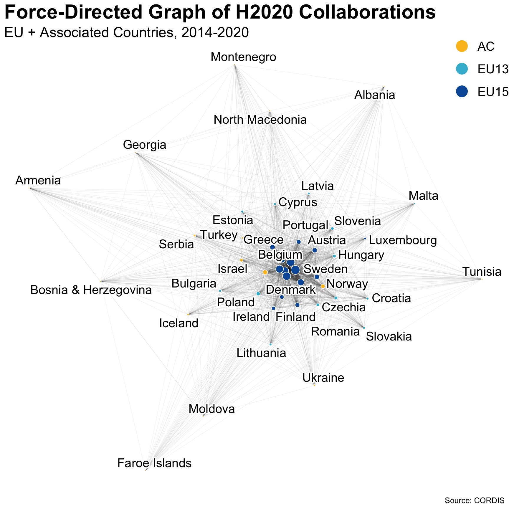
Difficult to perceive differences between the core countries.
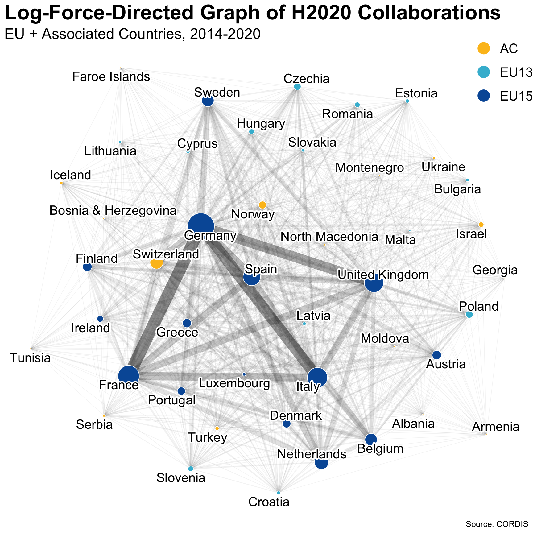
Log-Scaled Weighting
# recalculating point coordinates using "log(edge weights)"
point_coordinates <- igraph::layout_with_fr(g, weights = log(edge_weight))
colnames(point_coordinates) <- c("x", "y")

nodes <-
  point_coordinates %>%
  as_tibble() %>%
  mutate(country = names(igraph::V(g))) %>%
  left_join(info_country, by = "country") %>%
  mutate(
    status = str_to_upper(group),
    country_name = countrycode(country, "eurostat", "country.name"),
    s = node_size
  ) %>%
  arrange(s)

edges <- get.data.frame(g) %>%
  as_tibble() %>%
  left_join(select(nodes, x:country), by = c("from" = "country")) %>%
  rename(from_x = x, from_y = y) %>%
  left_join(select(nodes, x:country), by = c("to" = "country")) %>%
  rename(to_x = x, to_y = y) %>%
  mutate(s = weight) %>%
arrange(s)ggplot() +
geom_segment(
data = edges,
aes(
x = from_x,
xend = to_x,
y = from_y,
yend = to_y,
size = s,
colour = s
),
show.legend = FALSE
) +
scale_color_gradient(low = rgb(0, 0, 0, .05),
high = rgb(0, 0, 0, .45)) +
geom_point(
data = nodes,
aes(x, y, size = s, fill = status),
pch = 21,
colour = "white"
) +
scale_fill_manual(values = colorhunt) +
scale_size(range = c(.25, 15)) +
guides(
fill = guide_legend(override.aes = list(size = 7, shape = 21)),
color = "none",
size = "none") +
geom_text_repel(
data = nodes,
aes(x, y, label = country_name),
size = 5.5,
segment.color = NA,
bg.color = "white",
bg.r = 0.15
) +
labs(title = "Log-Force-Directed Graph of H2020 Collaborations",
subtitle = "EU + Associated Countries, 2014-2020",
caption = "Source: CORDIS") +
theme_bw() +
theme(
plot.title.position = "plot",
plot.title = element_text(size = 25, face = "bold"),
plot.subtitle = element_text(size = 18),
plot.caption = element_text(size = 10),
legend.position = c(.95, .95),
legend.title = element_blank(),
legend.text = element_text(size = 16),
legend.key.size = unit(2, "lines"),
axis.title = element_blank(),
axis.text = element_blank(),
axis.ticks = element_blank(),
axis.line = element_blank(),
panel.grid.major = element_blank(),
panel.grid.minor = element_blank(),
panel.border = element_blank(),
panel.background = element_blank()
)
Log-Scaled w/ Contribution Weighting
df_collab %>%
  ggplot(aes(role, contribution)) +
  geom_boxplot() +
  scale_y_log10(labels = label_number(accuracy = 1)) +
  coord_flip() +
  theme_bw()
Re-calculating weights using country-specific financial contributions:
pivot <- df_collab %>%
  group_by(rcn, country) %>%
  summarise(n = sum(contribution, na.rm = TRUE),
            .groups = "drop") %>%
  pivot_wider(names_from = country,
              values_from = n,
              values_fill = 0)

collaborations <- pivot %>%
  select(-rcn) %>%
  as.matrix() %>%
  crossprod()

g_collab <- collaborations %>%
  igraph::graph_from_adjacency_matrix(mode = "undirected",
                                      weighted = TRUE)
# remove same-country collaboration (diagonal 2x)
g <- igraph::simplify(g_collab)
node_size <-   igraph::strength(g) # ignore same-country collaboration
edge_weight <- igraph::E(g)$weight

point_coordinates <- igraph::layout_with_fr(g, weights = log(edge_weight))
colnames(point_coordinates) <- c("x", "y")

nodes <-
  point_coordinates %>%
  as_tibble() %>%
  mutate(country = names(igraph::V(g))) %>%
  left_join(info_country, by = "country") %>%
  mutate(
    status = str_to_upper(group),
    country_name = countrycode(country, "eurostat", "country.name"),
    s = node_size
  ) %>%
  arrange(s)

edges <- get.data.frame(g) %>%
  as_tibble() %>%
  left_join(select(nodes, x:country), by = c("from" = "country")) %>%
  rename(from_x = x, from_y = y) %>%
  left_join(select(nodes, x:country), by = c("to" = "country")) %>%
  rename(to_x = x, to_y = y) %>%
  mutate(s = weight) %>%
arrange(s)ggplot() +
geom_segment(
data = edges,
aes(
x = from_x,
xend = to_x,
y = from_y,
yend = to_y,
size = s,
colour = s
),
show.legend = FALSE
) +
scale_color_gradient(low = rgb(0, 0, 0, .05),
high = rgb(0, 0, 0, .45)) +
geom_point(
data = nodes,
aes(x, y, size = s, fill = status),
pch = 21,
colour = "white"
) +
scale_fill_manual(values = colorhunt) +
scale_size(range = c(.25, 15)) +
guides(
fill = guide_legend(override.aes = list(size = 7, shape = 21)),
color = "none",
size = "none") +
geom_text_repel(
data = nodes,
aes(x, y, label = country_name),
size = 5.5,
segment.color = NA,
bg.color = "white",
bg.r = 0.15
) +
labs(title = "Log-Force-Directed Graph of H2020 Collaborations",
subtitle = "EU + Associated Countries, 2014-2020",
caption = "Source: CORDIS") +
theme_bw() +
theme(
plot.title.position = "plot",
plot.title = element_text(size = 25, face = "bold"),
plot.subtitle = element_text(size = 18),
plot.caption = element_text(size = 10),
legend.position = c(.95, .95),
legend.title = element_blank(),
legend.text = element_text(size = 16),
legend.key.size = unit(2, "lines"),
axis.title = element_blank(),
axis.text = element_blank(),
axis.ticks = element_blank(),
axis.line = element_blank(),
panel.grid.major = element_blank(),
panel.grid.minor = element_blank(),
panel.border = element_blank(),
panel.background = element_blank()
)
# re-calculate layout on log-scale of edge weight
# spread core:
point_coordinates <- g %>%
  #  edge weight
  igraph::layout_with_fr(weights = log(edge_weight))
colnames(point_coordinates) <- c("x", "y")

nodes <-
  point_coordinates %>%
  as_tibble() %>%
  mutate(country = names(igraph::V(g))) %>%
  left_join(info_country, by = "country") %>%
  mutate(
    status = str_to_upper(group),
    country_name = countrycode(country, "eurostat", "country.name"),
    s = node_size
  ) %>%
  arrange(s)

edges <- g %>%
  get.data.frame() %>%
  as_tibble() %>%
  left_join(select(nodes, x:country), by = c("from" = "country")) %>%
  rename(from_x = x, from_y = y) %>%
  left_join(select(nodes, x:country), by = c("to" = "country")) %>%
  rename(to_x = x, to_y = y) %>%
  mutate(s = (weight / 1000) ^ 2.5) %>% # ad-hoc
  arrange(s)

# separate rules to approach Nature's representation
threshold <- 1 # ad-hoc
core_edges <- edges %>%
  filter(s > threshold)
outer_edges <- edges %>%
  filter(s <= threshold)
outer_edges_reversed <- outer_edges %>%
  rename(from = to, to = from) %>%
  select(from, everything())
outer_edges <- outer_edges %>%
  bind_rows(outer_edges_reversed) %>%
  anti_join(core_edges, by = "from") %>%
  anti_join(core_edges, by = c("from" = "to")) %>%
  group_by(from) %>%
  top_n(1, s) %>%
  mutate(s = 1)

edges <- core_edges %>%
  bind_rows(outer_edges) %>%
  arrange(s) # plot stronger edges last
Pop., Collab., Contrib.
Below, a log-log scale updated representation of Figure 2 from Network dynamics in collaborative research in the EU, 2003–2017.
population_table <- wbstats::wb_data(
  indicator = "SP.POP.TOTL",
  country = countrycode(pull(info_country, country), "eurostat", "iso2c"),
  start_date = 2017,
  end_date = 2017
) %>%
  clean_names() %>%
  select(iso2c, population = sp_pop_totl)

funding <- df_collab %>%
  group_by(country) %>%
  summarise(contrib = sum(contribution, na.rm = TRUE),
            .groups = "drop")

collaborations <- df_collab %>%
  # keep group information
  group_by(group, country) %>%
  summarise(n = n(),
            .groups = "drop") %>%
  # for world bank compatibility
  mutate(
    status = str_to_upper(group),
    iso2c = countrycode(country, "eurostat", "iso2c"),
    country_name = countrycode(country, "eurostat", "country.name")) %>%
  left_join(population_table, by = "iso2c") %>%
left_join(funding, by = "country")ggplot(aes(population, n, label = country_name, col = status),
data = collaborations) +
geom_smooth(
method = "lm",
se = FALSE,
col = "gray75",
linetype = "dotted",
size = .5
) +
geom_point(size = 3, alpha = .8) +
geom_text_repel(
size = 5,
force = 2,
segment.alpha = 0.5,
bg.color = rgb(1, 1, 1, .5),
bg.r = 0.15,
show.legend = FALSE
) +
scale_color_manual(values = colorhunt) +
scale_x_log10(labels = label_number(accuracy = 1, scale = 1e-6)) +
scale_y_log10(labels = label_number(accuracy = 1, scale = 1e-3)) +
labs(
title = "H2020 Collaborations and Population",
subtitle = "Shown in log-log scale",
caption = "Source: CORDIS, World Bank",
color = element_blank(),
x = "Population (mio)",
y = "No. Collaborations (k)"
) +
theme_minimal() +
theme(
plot.title.position = "plot",
legend.position = c(.1, .96),
legend.direction = "horizontal",
legend.key.size = unit(4, "mm"),
legend.background = element_rect(
linetype = "dotted",
fill = alpha("white", 1),
color = alpha("black", 0.25)
)
)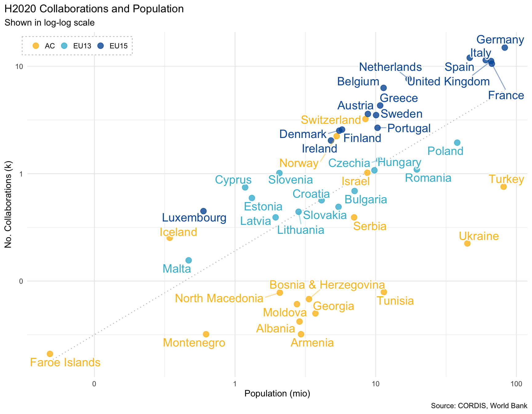
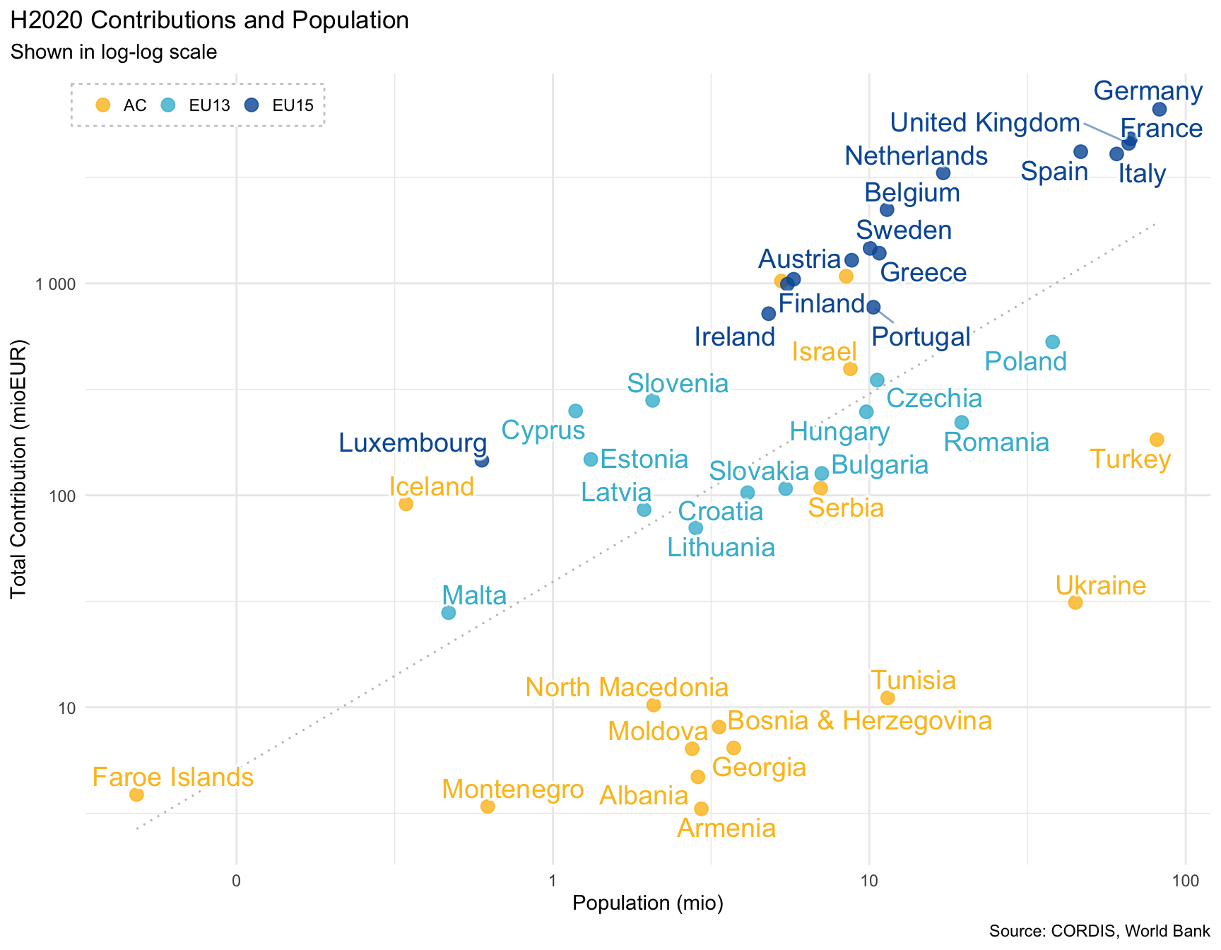
Related plots:
ggplot(aes(population, contrib, label = country_name, col = status),
       data = collaborations) +
  geom_smooth(
    method = "lm",
    se = FALSE,
    col = "gray75",
    linetype = "dotted",
    size = .5
  ) +
  geom_point(size = 3, alpha = .8) +
  geom_text_repel(
    size = 5,
    force = 2,
    segment.alpha = 0.5,
    bg.color = rgb(1, 1, 1, .5),
    bg.r = 0.15,
    show.legend = FALSE
  ) +
  scale_color_manual(values = colorhunt) +
  scale_x_log10(labels = label_number(accuracy = 1, scale = 1e-6)) +
  scale_y_log10(labels = label_number(accuracy = 1, scale = 1e-6)) +
  labs(
    title = "H2020 Contributions and Population",
    subtitle = "Shown in log-log scale",
    caption = "Source: CORDIS, World Bank",
    color = element_blank(),
    x = "Population (mio)",
    y = "Total Contribution (mioEUR)"
  ) +
  theme_minimal() +
  theme(
    plot.title.position = "plot",
    legend.position = c(.1, .96),
    legend.direction = "horizontal",
    legend.key.size = unit(4, "mm"),
    legend.background = element_rect(
      linetype = "dotted",
      fill = alpha("white", 1),
      color = alpha("black", 0.25)
    )
  )
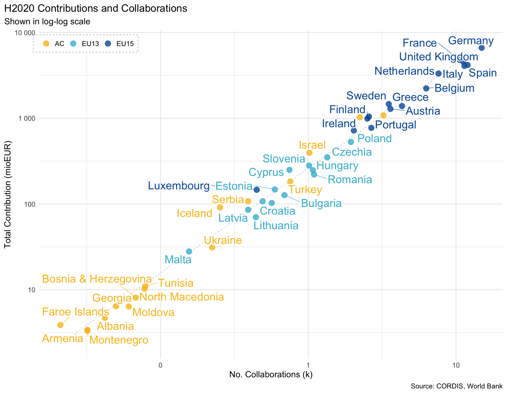
ggplot(aes(n, contrib, label = country_name, col = status),
       data = collaborations) +
  geom_smooth(
    method = "lm",
    se = FALSE,
    col = "gray75",
    linetype = "dotted",
    size = .5
  ) +
  geom_point(size = 3, alpha = .8) +
  geom_text_repel(
    size = 5,
    force = 2,
    segment.alpha = 0.5,
    bg.color = rgb(1, 1, 1, .5),
    bg.r = 0.15,
    show.legend = FALSE
  ) +
  scale_color_manual(values = colorhunt) +
  scale_x_log10(labels = label_number(accuracy = 1, scale = 1e-3)) +
  scale_y_log10(labels = label_number(accuracy = 1, scale = 1e-6)) +
  labs(
    title = "H2020 Contributions and Collaborations",
    subtitle = "Shown in log-log scale",
    caption = "Source: CORDIS, World Bank",
    color = element_blank(),
    x = "No. Collaborations (k)",
    y = "Total Contribution (mioEUR)"
  ) +
  theme_minimal() +
  theme(
    plot.title.position = "plot",
    legend.position = c(.1, .96),
    legend.direction = "horizontal",
    legend.key.size = unit(4, "mm"),
    legend.background = element_rect(
      linetype = "dotted",
      fill = alpha("white", 1),
      color = alpha("black", 0.25)
    )
  )