Gender and Other Potential Biases in Peer Review: Analysis of 38,250 External Peer Review Reports

Data Analysis Notebook

Synopsis

This notebook provides additional material to a preprint of a manuscript and a conference abstract presented at the 5th International Congress on Peer Review and Scientific Publication.

Data

We analyzed review scores provided by external reviewers evaluating the overall quality of grant applications submitted to SNSF project funding between 2009 and 2016. Our goal is to investigate possible scoring biases by exploring how scores distribute under different conditions. We explored differences in score distributions according to the origin of the review (Switzerland/international), the gender of the applicant and of the reviewer (male/female), and the source of nomination of the reviewer (applicant/SNSF).

The dataset contains 38’250 reviews of 12’294 unique grant applications submitted by 5’832 unique applicants and evaluated by 26’829 unique external reviewers between 2009 and 2016. The average number of reviews per grant application was 3.11, applicants submitted an average of 2.11 grant applications and reviewers reviewed an average of 1.42 applications. The review scores (overall_score) consist of the following six-level rating scale: poor (1), fair (2) average (3), good (4), excellent (5), and outstanding (6). The following table gives characteristics of the applicants on the date of their first submission of a project grant proposal (Table 1 of the manuscript). Figure 1 shows how the amount of female applicants increased over time compared to male applicants. It also shows the average ratio of female external reviewers per project. This last ratio depends however strongly on the research topic (see Figure 2).

	Female applicants	Male applicants
	(n = 1306, 22.44)	(n = 4514, 77.56)
Age (mean, SD)	46.23 (8.27)	48.24 (8.63)
applicant_affiliation
ETH Domain	219 (16.77%)	1195 (26.47%)
Other	224 (17.15%)	481 (10.66%)
Universities	863 (66.08%)	2838 (62.87%)
applicant_nationality
ch	733 (56.13%)	2618 (58%)
int	573 (43.87%)	1896 (42%)
research_topic
Architecture	56 (4.29%)	146 (3.23%)
Biology	129 (9.88%)	611 (13.54%)
Chemistry	76 (5.82%)	378 (8.37%)
Economics	84 (6.43%)	290 (6.42%)
Engineering	74 (5.67%)	527 (11.67%)
Geology	24 (1.84%)	144 (3.19%)
History	68 (5.21%)	209 (4.63%)
Linguistics	102 (7.81%)	203 (4.5%)
Math./Physics	56 (4.29%)	491 (10.88%)
Medicine	317 (24.27%)	1029 (22.8%)
Psychology	164 (12.56%)	223 (4.94%)
Sociology	156 (11.94%)	263 (5.83%)
call_end_date
2009-04-01	27 (2.07%)	118 (2.61%)
2009-10-01	45 (3.45%)	164 (3.63%)
2010-04-01	35 (2.68%)	150 (3.32%)
2010-10-01	49 (3.75%)	187 (4.14%)
2011-04-01	52 (3.98%)	163 (3.61%)
2011-10-01	52 (3.98%)	195 (4.32%)
2012-04-01	58 (4.44%)	205 (4.54%)
2012-10-01	62 (4.75%)	249 (5.52%)
2013-04-01	78 (5.97%)	313 (6.93%)
2013-10-01	88 (6.74%)	309 (6.85%)
2014-04-01	117 (8.96%)	349 (7.73%)
2014-10-01	153 (11.72%)	368 (8.15%)
2015-04-01	132 (10.11%)	459 (10.17%)
2015-10-01	170 (13.02%)	609 (13.49%)
2016-04-01	188 (14.4%)	676 (14.98%)
applicant_continent_notCH
Africa	1 (0.08%)	13 (0.29%)
Americas	39 (2.99%)	126 (2.79%)
Asia	14 (1.07%)	54 (1.2%)
Europe (not CH)	517 (39.59%)	1695 (37.55%)
Oceania	2 (0.15%)	7 (0.16%)
Switzerland	733 (56.13%)	2618 (58%)
NA	NA	1 (0.02%)

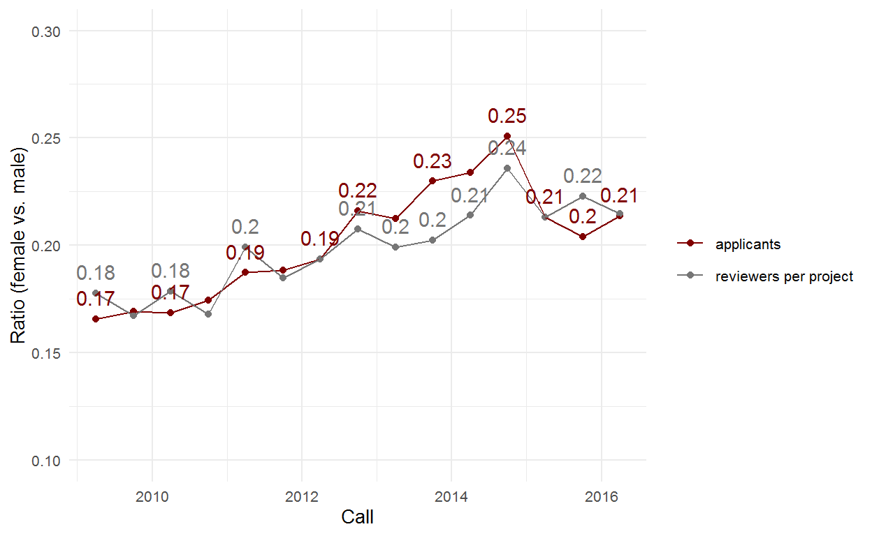
Figure 1: Ratio of females among all the applicants over time and ratio of female external reviewers per grant application.

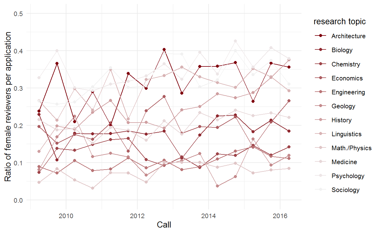
Figure 2: Ratio of females reviewers per grant application over time depending on the research topic.

17.8% of the grant applications had only male external reviewers, while 1.05% had only female external reviewers. For the applications rated by at least one male and one female reviewer, the male reviewer(s) gave a score which was on average 0.04 points higher than the score attributed by the female reviewer(s).

Exploratory Data Analysis

Score Frequency Distributions

Visual inspection of the frequency distributions of review scores indicate overall negative skweness.

Figures 3 and 4 show that the skweness is strongest for review scores attributed by applicant-nominated reviewers (Figure 3). Figure 4 also reveals that the relative frequency of outstanding review scores from international-based reviewers is roughly double of that from Swiss-based reviewers.

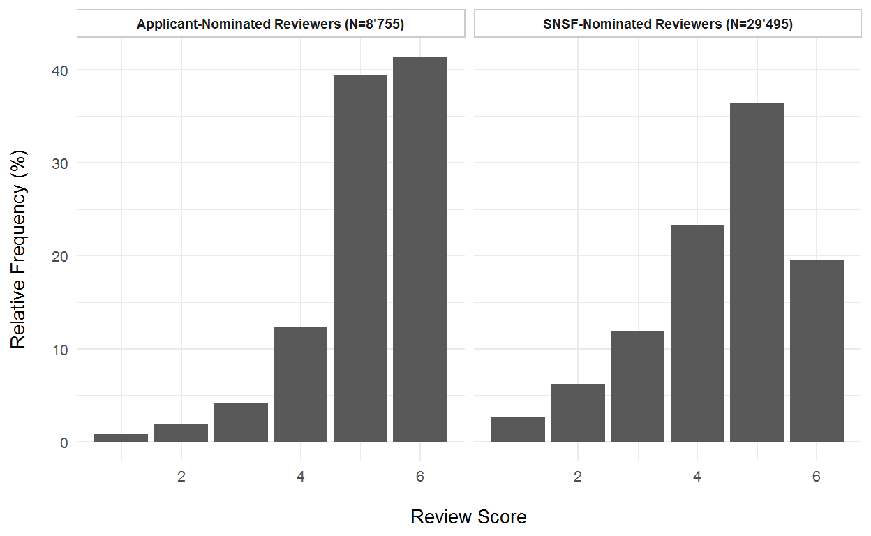
Figure 3: Frequency distributions of external review scores by source of nomination of the reviewer. Applicant-nominated reviewers on the left, SNSF-nominated reviewers on the right.

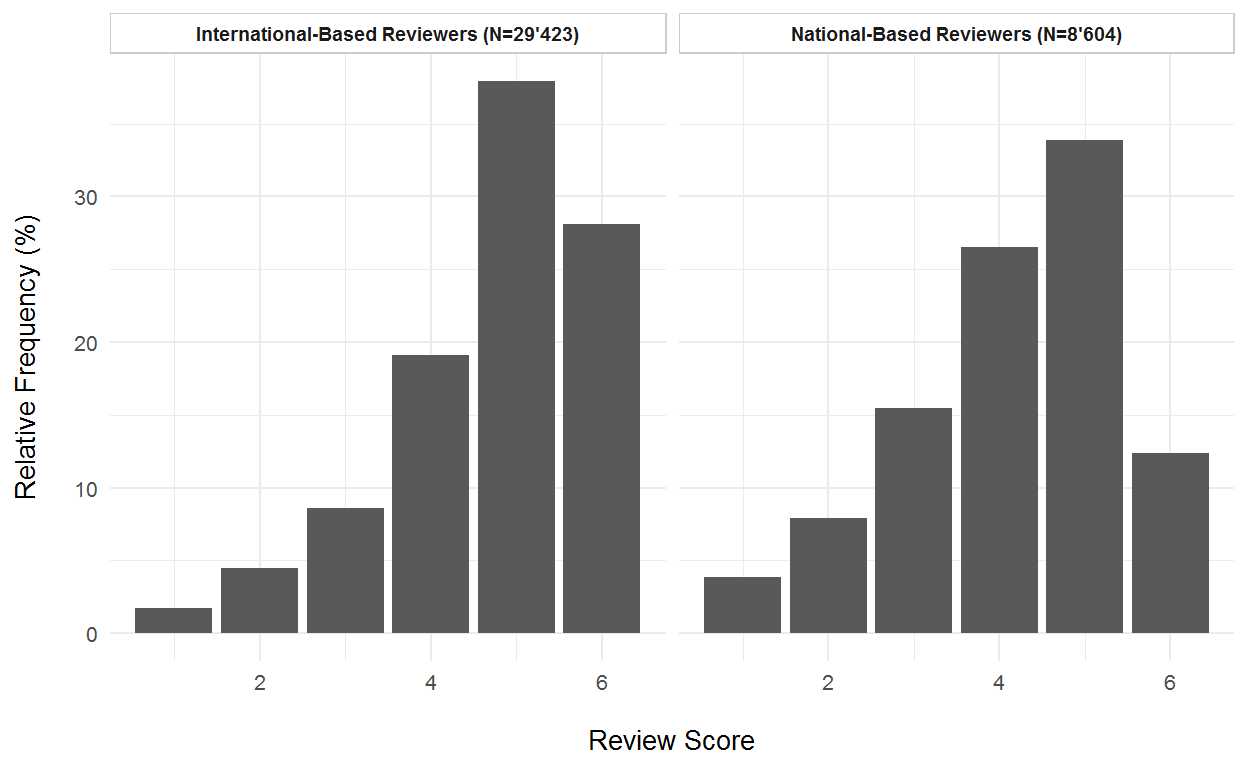
Figure 4: Frequency distributions of external review scores by country of affiliation of the reviewer. International-based reviewers on the left, Swiss-based reviewers on the right.

The gender of the applicants also appears to have an influence on review scores’ distribution. Figure 5 shows a more negative skweness of the review scores’ distribution for male applicant than for female applicants.

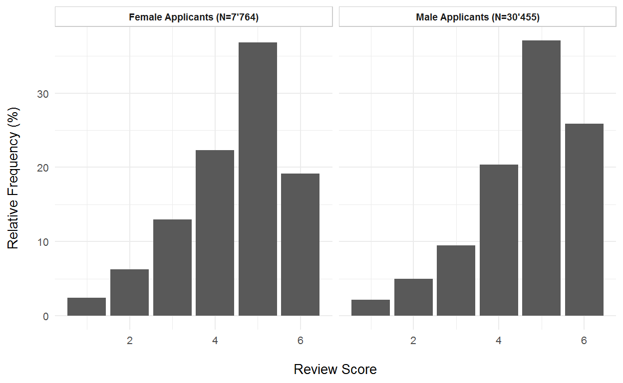
Figure 5: Frequency distributions of external review scores by gender of the principal applicants.

Interestingly, gender of reviewers follow a similar pattern. Figure 6 shows that the skweness also seems to be more negative for review scores given by male reviewers than by female reviewers. This indicates that both the gender of applicants and reviewers likely have an influence on review scores’ distribution. The Table 1 shows the same information in form of a table.

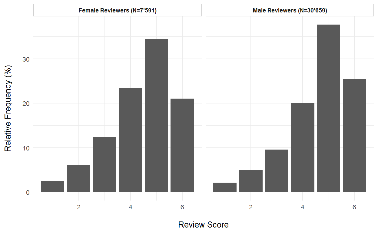
Figure 6: Frequency distributions of external review scores by gender of the reviewers.

Table 1: Average and median overall score depending on certain characteristics of the applicants and review process, together with their standard deviation and interquartile range.

	Average overall score (SD)	Median overall score (IQR)
Applicant-Nominated Reviewers (N=8’755)	5.12 (1)	5 (1)
SNSF-Nominated Reviewers (N=29’495)	4.43 (1.25)	5 (1)
International-Based Reviewers (N=29’423)	4.71 (1.19)	5 (2)
National-Based Reviewers (N=8’604)	4.16 (1.28)	4 (2)
Female Applicants (N=7’764)	4.42 (1.25)	5 (1)
Male Applicants (N=30’455)	4.63 (1.22)	5 (2)
Female Reviewers (N=7’591)	4.44 (1.26)	5 (1)
Male Reviewers (N=30’659)	4.63 (1.22)	5 (2)

To follow on gender, we show, in Figure 7, summary statistics of the review scores by gender of the applicant and by research topic. For example. in Mathematics and Physics, male applicants receive outstandingly high review scores on average.

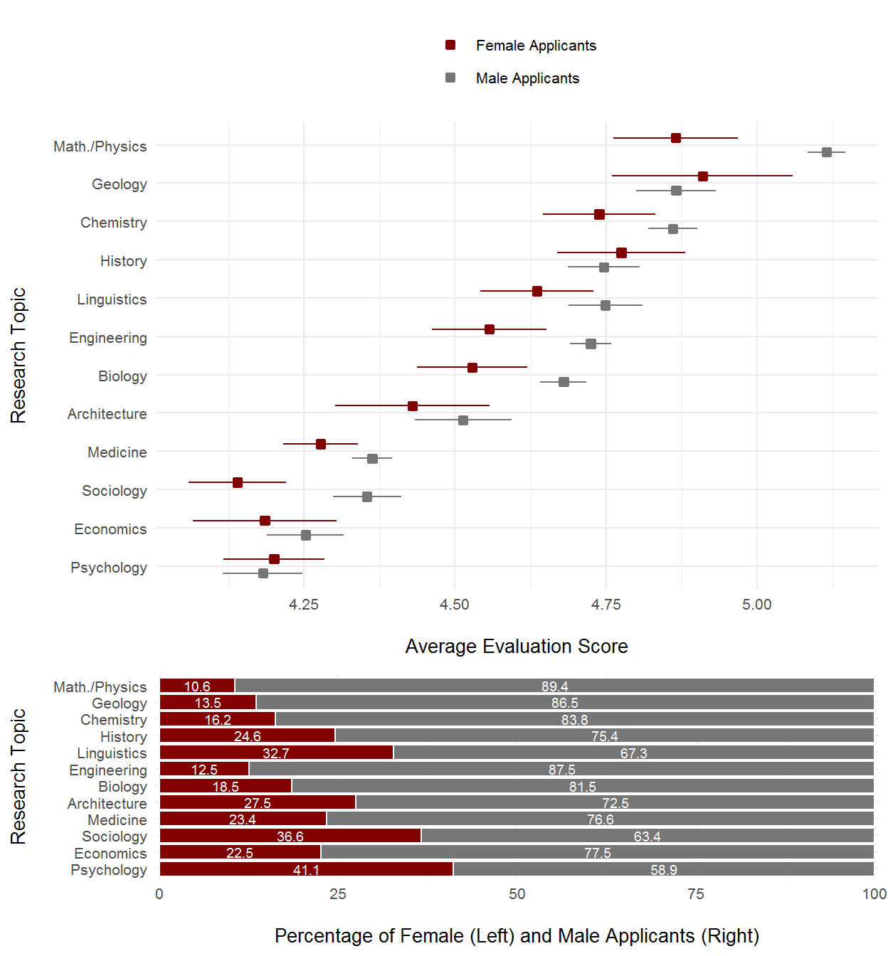
Figure 7: Upper panel: Mean review scores by research topic of the grant applications for both female and male applicants. Horizontal lines indicate Wald confidence intervals of the mean. Lower panel: Proportions of female and male applicants by research topic.

Figure 8 shows summary statistics of the review scores by gender and by age group of the applicants. This representation reveals a clearer distinction in the average review scores between the two genders. Figure 8 also presents the “leaky pipeline” by plotting the share of female grant applicants for each age class in the bottom-right panel of the figure. Figure 9 simply zooms into the previous one, by deleting the group with very low counts.

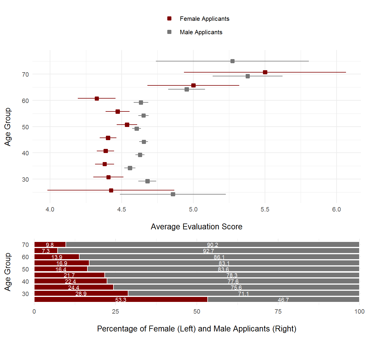
Figure 8: Upper panels: mean review scores by age group for both female (top) and male (bottom) applicants. Horizontal lines indicate the Wald confidence interval of the mean. Lower panel: Proportions of female and male applicants per age group.

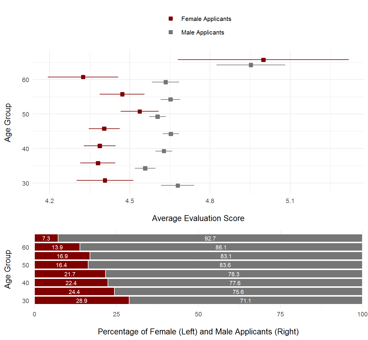
Figure 9: Upper panels: mean review scores by age group for both female (top) and male (bottom) applicants. Horizontal lines indicate the Wald confidence interval of the mean. Lower panel: Proportions of female and male applicants per age group. This figure does not include the age groups with very low counts to facilitate the interpretation.

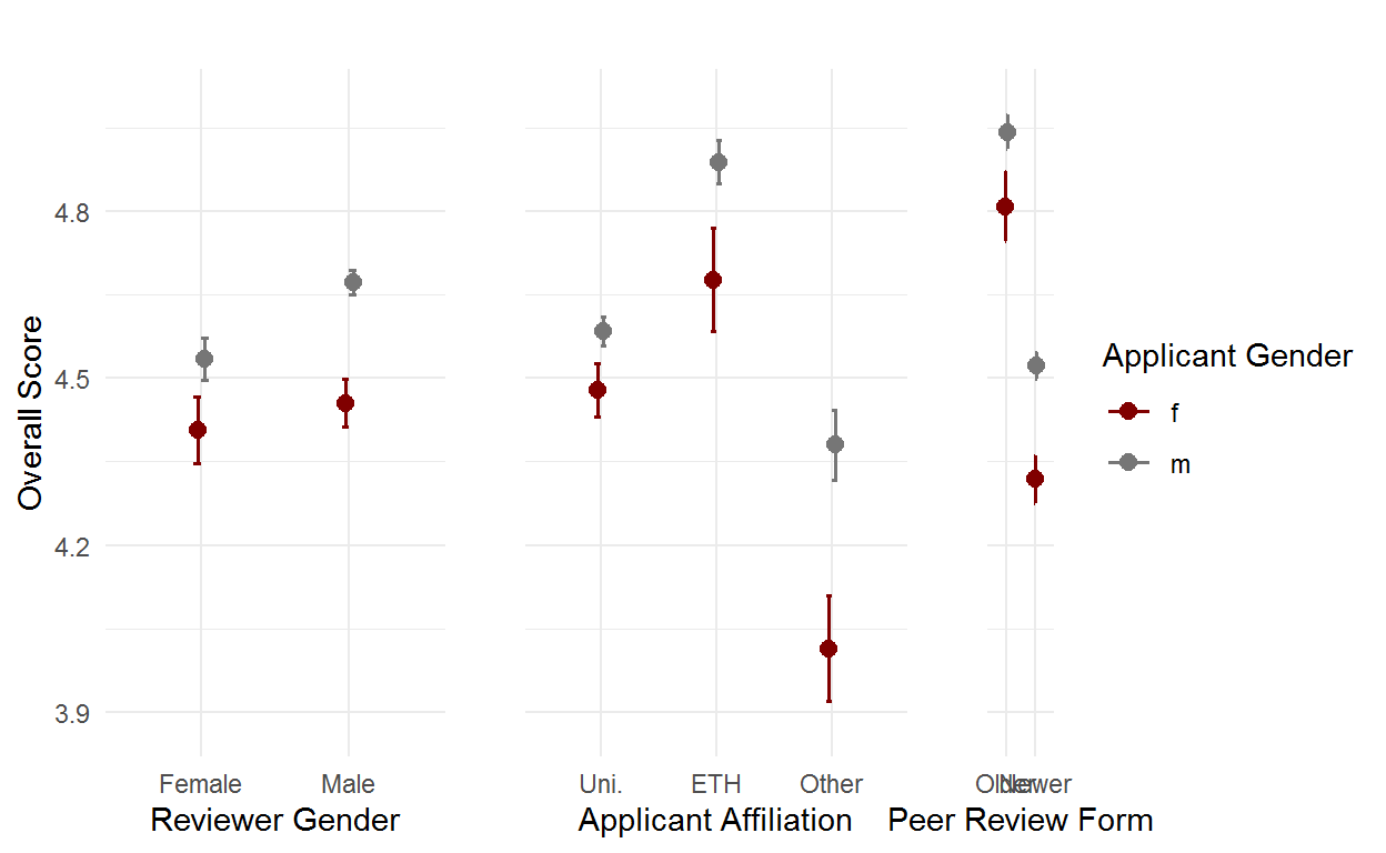
In Figure 10, we show summary statistics of the review scores by gender and by affiliation of the applicants. Grants submitted by researchers from the ETH Domain receive higher average scores than applications from Cantonal Universities or from Other Research Institutes. Gender differences are more easily noticeable in the ETH Domain and Other Research Institutions than in Cantonal Universities.

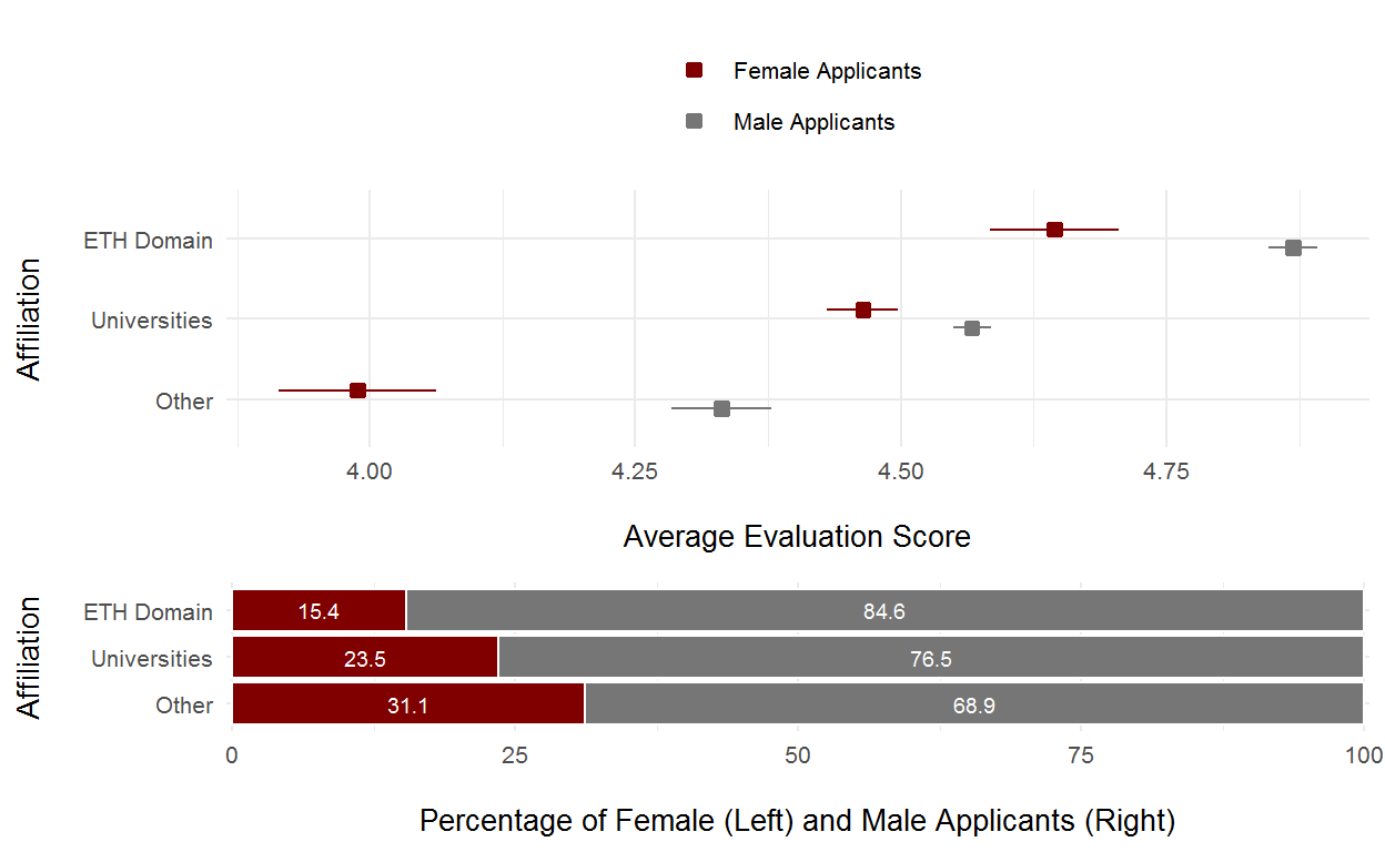
Figure 10: Upper panels: Mean review scores by the affiation of the applicants. Point range indicates the Wald confidence interval of the mean. Lower panel: Proportions of female and male applicants by affiliation.

Another possible source of bias could be the nationality of grant applicants. In Figure 11, we again show summary statistics of the review scores by gender and by nationality if the applicants. Both national and foreign male applicants receive higher reviews scores than their female counterparts, on average, with foreign national scoring slightly above Swiss nationals on average.

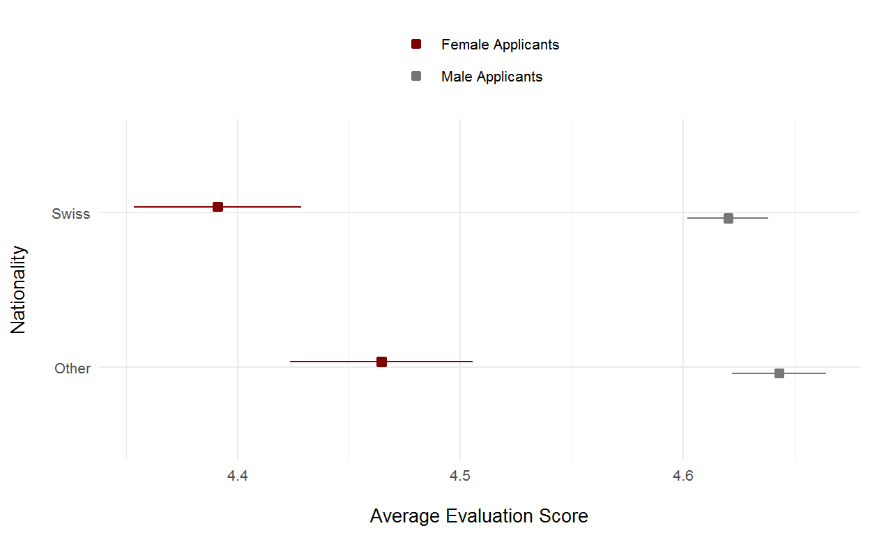
Figure 11: Mean review scores by the nationality of the applicant type. Point range indicates the Wald confidence interval of the mean.

Last, Figure 12 illustrates the introduction of new guidelines for reviewers in 2011-10-01. Grant applications submitted before 2011-10-01 show significantly higher average scores than the more recent applications. We account for this shift in the distribution of review scores with a dummy variable (call_cut) which groups grant applications according to whether they were submitted before or after the introduction of the newer reviewing guidelines.

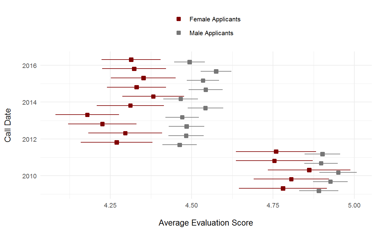
Figure 12: Mean review scores by call deadline. Point range indicates Wald confidence intervals of the mean.

Estimating the Effect of Each Variable

To quantify the effect of each variable on the observed mean differences, we fit the data points to a linear mixed effects model (Bates et al. 2015). This type of model extends the linear model in that it accounts for both random and fixed types of effects (Harrison et al. 2018) and is often preferred over ordinal mixed effects models when the dependent variable has 5 or more levels.

An ordinal mixed effects models are also appropriate when the target variable is not continuous (Christensen 2018).

First, we explore which random effect to include by adding random effects step-wise and measuring the relative gain in predictive power using Akaike’s Information Criterion (AIC) and Chi-squared comparisons. Then, we proceed by adding the fixed effects.

Data manipulations before modelling

To make a comparison of the later univariate or crude estimates and multivariate or adjusted estimates feasible we proceed to a ‘complete case’ analysis. Otherwise the models with variables without any missings are developed on the whole dataset with 38’250 observations while the full model includes variable with some missings leading to a development dataset with only 37’979 reviews. Hence, we will reduce the dataset used for all modelling to the set of 37’979 (99.3%) observations.
A second small data manipulation is the releveling of the two factors in the adjusted model, ‘applicant_affiliation’ and ‘research_topic’. The reference of the factors will simply be the level with the highest count, which is ‘Universities’ for the affiliation and ‘Medicine’ for the research topic. The following Table presents some summary statistics of this complete data set.

Random Effects

As already mentioned, each grant application typically receives more than one independent review, with each reviewer being able to review more than one grant application over the time period considered.

We start by explaining the overall score (overall_score) as a function of the dummy variable call_cut, accounting for introduction of new reviewing guidelines in 2011-10-01, and two random effects, one accounting for the project_id (unique identifier of a grant application), the other accounting for the reviewer_id (unique identifier a reviewer). In R, we write a first model (model_1) as follows:

lme4::lmer(score ~ call_cut +
                   (1|project_id) + (1|reviewer_id))

We include the fixed effect of the dummy variable call_cut in all three models to ensure compatibility in comparing models one and two with model three.

Summary statistics for model_1.

	overall score
Coefficient	Estimates	SE	t-Statistic	P-Value
(Intercept)	4.92 (4.89 – 4.94)	0.01	353.67	<0.001
newer	-0.43 (-0.47 – -0.40)	0.02	-27.17	<0.001
Random Effects
σ2	0.69
τ00 reviewer_id	0.49
τ00 project_id	0.28
ICC	0.53
N project_id	12277
N reviewer_id	26614
Observations	37979
Marginal R2 / Conditional R2	0.026 / 0.539

In a second random effects model (model_2), we add a random effect accounting for the applicant_id (unique identifier of a grant applicant) to account for the fact that each applicant may submit more than one grant application. In R, the model is written as:

lme4::lmer(score ~ call_cut +
                   (1|project_id) + (1|reviewer_id) + (1|applicant_id))

Summary statistics for model_2.

	overall score
Coefficient	Estimates	SE	t-Statistic	P-Value
(Intercept)	4.91 (4.89 – 4.94)	0.01	340.02	<0.001
newer	-0.44 (-0.47 – -0.41)	0.02	-29.12	<0.001
Random Effects
σ2	0.70
τ00 reviewer_id	0.47
τ00 project_id	0.08
τ00 applicant_id	0.23
ICC	0.53
N applicant_id	5819
N project_id	12277
N reviewer_id	26614
Observations	37979
Marginal R2 / Conditional R2	0.026 / 0.542

Last, in a third random effects model (model_3), we add a random effect accounting for the call_end_date, to account for any possible correlations across calls which might not be yet explained by the dummy variable call_cut:

lme4::lmer(score ~ call_cut +
                   (1|project_id) + (1|reviewer_id) + (1|applicant_id) +
                   (1|call_end_date))

Summary statistics for model_3.

	overall score
Coefficient	Estimates	SE	t-Statistic	P-Value
(Intercept)	4.91 (4.88 – 4.95)	0.02	272.44	<0.001
newer	-0.44 (-0.48 – -0.40)	0.02	-21.85	<0.001
Random Effects
σ2	0.70
τ00 reviewer_id	0.47
τ00 project_id	0.08
τ00 applicant_id	0.23
τ00 call_end_date	0.00
ICC	0.53
N call_end_date	15
N applicant_id	5819
N project_id	12277
N reviewer_id	26614
Observations	37979
Marginal R2 / Conditional R2	0.026 / 0.542

An analysis of the random effects of the three models shows that the second model significantly reduces the residual sum of squares of the first model (see Table 2).

Table 2: Pairwise comparison of the residual sum of squares between the first and second models.

Model	Df	AIC	BIC	logLik	deviance	Chisq	Df	Pr(>Chisq)
model_1	5	118462.7	118505.4	-59226.33	118452.7	NA	NA	NA
model_2	6	117552.2	117603.5	-58770.11	117540.2	912.4297	1	0

The third model, however, accounting for an extra random effect for the call_end_date does not improve the second model significantly (see Table 3). We will therefore use the second model as the basis to measure possible fixed effects of remaining factors.

Table 3: Pairwise comparison of the residual sum of squares between the second and third models.

Model	Df	AIC	BIC	logLik	deviance	Chisq	Df	Pr(>Chisq)
model_2	6	117552.2	117603.5	-58770.11	117540.2	NA	NA	NA
model_3	7	117551.8	117611.6	-58768.88	117537.8	2.473346	1	0.1157912

Fixed Effects

Using the model accounting for the random effects of both applicants and reviewers, we first look at the crude fixed effects regarding:

1. the origin of the review

lme4::lmer(score ~ call_cut + review_origin +
                   (1|project_id) + (1|reviewer_id) + (1|applicant_id))

Summary statistics for the crude effect related to the country of affiliation of the reviewer.

	overall score
Coefficient	Estimates	SE	t-Statistic	P-Value
(Intercept)	5.03 (5.00 – 5.06)	0.01	342.40	<0.001
Reviewer: Swiss-Based	-0.53 (-0.56 – -0.49)	0.02	-30.12	<0.001
Call Cut: 2009–2011	-0.46 (-0.49 – -0.44)	0.01	-31.27	<0.001
Random Effects
σ2	0.71
τ00 reviewer_id	0.43
τ00 project_id	0.08
τ00 applicant_id	0.21
ICC	0.50
N applicant_id	5819
N project_id	12277
N reviewer_id	26614
Observations	37979
Marginal R2 / Conditional R2	0.056 / 0.530

2. the gender of the applicant

lme4::lmer(score ~ call_cut + applicant_gender +
                   (1|project_id) + (1|reviewer_id) + (1|applicant_id))

Summary statistics for the crude effect related to the gender of the applicant.

	overall score
Coefficient	Estimates	SE	t-Statistic	P-Value
(Intercept)	4.77 (4.72 – 4.81)	0.02	208.19	<0.001
Applicant: Male	0.18 (0.14 – 0.23)	0.02	8.31	<0.001
Call Cut: 2009–2011	-0.43 (-0.46 – -0.40)	0.01	-28.89	<0.001
Random Effects
σ2	0.70
τ00 reviewer_id	0.47
τ00 project_id	0.08
τ00 applicant_id	0.23
ICC	0.53
N applicant_id	5819
N project_id	12277
N reviewer_id	26614
Observations	37979
Marginal R2 / Conditional R2	0.030 / 0.542

3. the gender of the reviewer

lme4::lmer(score ~ call_cut + reviewer_gender +
                   (1|project_id) + (1|reviewer_id) + (1|applicant_id))

Summary statistics for the crude effect related to the gender of the reviewer.

	overall score
Coefficient	Estimates	SE	t-Statistic	P-Value
(Intercept)	4.82 (4.78 – 4.86)	0.02	243.69	<0.001
Reviewer: Male	0.11 (0.08 – 0.15)	0.02	6.84	<0.001
Call Cut: 2009–2011	-0.43 (-0.46 – -0.41)	0.01	-28.99	<0.001
Random Effects
σ2	0.70
τ00 reviewer_id	0.47
τ00 project_id	0.08
τ00 applicant_id	0.23
ICC	0.53
N applicant_id	5819
N project_id	12277
N reviewer_id	26614
Observations	37979
Marginal R2 / Conditional R2	0.028 / 0.542

4. reviewer’s nomination source

lme4::lmer(score ~ call_cut + nomination_type +
                   (1|project_id) + (1|reviewer_id) + (1|applicant_id))

Summary statistics for the crude effect related to the source of nomination of the reviewer.

	overall score
Coefficient	Estimates	SE	t-Statistic	P-Value
(Intercept)	5.31 (5.27 – 5.34)	0.02	303.32	<0.001
Nomination: SNSF	-0.53 (-0.56 – -0.50)	0.01	-37.87	<0.001
Call Cut: 2009–2011	-0.41 (-0.44 – -0.38)	0.01	-27.85	<0.001
Random Effects
σ2	0.70
τ00 reviewer_id	0.42
τ00 project_id	0.08
τ00 applicant_id	0.20
ICC	0.50
N applicant_id	5819
N project_id	12277
N reviewer_id	26614
Observations	37979
Marginal R2 / Conditional R2	0.060 / 0.534

(5. the age of applicant)

lme4::lmer(score ~ applicant_age + call_cut +
                   (1|project_id) + (1|reviewer_id) + (1|applicant_id))

Summary statistics for the crude effect related to the age of the applicant.

	overall score
Coefficient	Estimates	SE	t-Statistic	P-Value
(Intercept)	4.66 (4.56 – 4.76)	0.05	89.98	<0.001
Applicant Age	0.06 (0.03 – 0.08)	0.01	5.09	<0.001
Call Cut: 2009–2011	-0.45 (-0.48 – -0.42)	0.02	-29.57	<0.001
Random Effects
σ2	0.70
τ00 reviewer_id	0.47
τ00 project_id	0.08
τ00 applicant_id	0.23
ICC	0.53
N project_id	12277
N reviewer_id	26614
N applicant_id	5819
Observations	37979
Marginal R2 / Conditional R2	0.028 / 0.543

(6. the affiliation of applicant)

lme4::lmer(score ~ applicant_affiliation + call_cut +
                   (1|project_id) + (1|reviewer_id) + (1|applicant_id))

Summary statistics for the crude effect related to the affiliation of the applicant.

	overall score
Coefficient	Estimates	SE	t-Statistic	P-Value
(Intercept)	4.86 (4.83 – 4.89)	0.02	309.43	<0.001
Applicant Affil.: ETH Domain	0.30 (0.26 – 0.34)	0.02	13.89	<0.001
Applicant Affil.: Other	-0.24 (-0.30 – -0.19)	0.03	-8.51	<0.001
Call Cut: 2009–2011	-0.43 (-0.46 – -0.40)	0.01	-28.66	<0.001
Random Effects
σ2	0.70
τ00 reviewer_id	0.47
τ00 project_id	0.08
τ00 applicant_id	0.21
ICC	0.52
N project_id	12277
N reviewer_id	26614
N applicant_id	5819
Observations	37979
Marginal R2 / Conditional R2	0.045 / 0.540

To see whether there actually is an effect of the affiliation we seek for a single p-value for this varible by applying the anova function on the models with and without the specific variable.

Table 4: Pairwise comparison of the residual sum to judge wether applicant affiliation has an effect on the score (only crude effect, unadjusted).

Model	Df	AIC	BIC	logLik	deviance	Chisq	Df	Pr(>Chisq)
model0_affiliation_crude	6	117552.2	117603.5	-58770.11	117540.2	NA	NA	NA
crude_5	8	117237.7	117306.1	-58610.86	117221.7	318.5097	2	0

(7. the nationality of applicant)

lme4::lmer(score ~ applicant_nationality + call_cut +
                   (1|project_id) + (1|reviewer_id) + (1|applicant_id))

Summary statistics for the crude effect related to the nationality of the applicant.

	overall score
Coefficient	Estimates	SE	t-Statistic	P-Value
(Intercept)	4.90 (4.87 – 4.94)	0.02	300.14	<0.001
App. Nationality: Foreign	0.03 (-0.01 – 0.06)	0.02	1.42	0.155
Call Cut: 2009–2011	-0.44 (-0.47 – -0.41)	0.02	-29.15	<0.001
Random Effects
σ2	0.70
τ00 reviewer_id	0.47
τ00 project_id	0.08
τ00 applicant_id	0.23
ICC	0.53
N project_id	12277
N reviewer_id	26614
N applicant_id	5819
Observations	37979
Marginal R2 / Conditional R2	0.026 / 0.542

(8. the research topic)

lme4::lmer(score ~ research_topic + call_cut +
                   (1|project_id) + (1|reviewer_id) + (1|applicant_id))

Summary statistics for the crude effect related to the research topic.

	overall score
Coefficient	Estimates	SE	t-Statistic	P-Value
(Intercept)	4.69 (4.65 – 4.73)	0.02	218.55	<0.001
Topic: Architecture	0.13 (0.03 – 0.24)	0.05	2.63	0.009
Topic: Biology	0.30 (0.24 – 0.36)	0.03	9.79	<0.001
Topic: Chemistry	0.46 (0.39 – 0.53)	0.04	13.05	<0.001
Topic: Economics	-0.09 (-0.17 – -0.01)	0.04	-2.21	0.027
Topic: Engineering	0.32 (0.25 – 0.38)	0.03	10.03	<0.001
Topic: Geology	0.50 (0.39 – 0.60)	0.05	9.24	<0.001
Topic: History	0.35 (0.27 – 0.44)	0.04	8.14	<0.001
Topic: Linguistics	0.30 (0.22 – 0.38)	0.04	7.13	<0.001
Topic: Math/Phys	0.68 (0.62 – 0.75)	0.03	20.52	<0.001
Topic: Psychology	-0.12 (-0.20 – -0.05)	0.04	-3.19	0.001
Topic: Sociology	-0.06 (-0.13 – 0.02)	0.04	-1.49	0.136
Call Cut: 2009–2011	-0.43 (-0.46 – -0.40)	0.01	-29.01	<0.001
Random Effects
σ2	0.71
τ00 reviewer_id	0.45
τ00 project_id	0.08
τ00 applicant_id	0.17
ICC	0.50
N project_id	12277
N reviewer_id	26614
N applicant_id	5819
Observations	37979
Marginal R2 / Conditional R2	0.068 / 0.533

To see whether there actually is an effect of the research topic we seek for a single p-value for this varible by applying the anova function on the models with and without the specific variable.

Table 5: Pairwise comparison of the residual sum to judge wether research topic type has an effect on the score (only crude effect, unadjusted).

Model	Df	AIC	BIC	logLik	deviance	Chisq	Df	Pr(>Chisq)
model0_topic_crude	6	117552.2	117603.5	-58770.11	117540.2	NA	NA	NA
crude_7	17	116829.4	116974.7	-58397.70	116795.4	744.8185	11	0

Finally, we look at the corresponding adjusted effects when accounting for the all factors together. In R, we write the model as follows:

lme4::lmer(score ~ call_cut +
                   nomination_type + research_topic +
                   applicant_gender + applicant_age +
                   applicant_affiliation + applicant_nationality +
                   review_origin + reviewer_gender +
                   (1|project_id) + (1|reviewer_id) + (1|applicant_id))

When accounting for the all factors, the adjusted effects regarding the origin of the reviews and source of nomination remain of the same order of magnitude as their corresponding unadjusted effects. The effects related to gender, however, nearly vanish. The adjusted effect of the gender of the applicants falls by more than 50% of its original unadjusted value, while the adjusted effect of the gender of the reviewer decreases by approximately 30% of its previous unadjusted value. This result indicates that most of the initially effect attributed to gender can be due to differences of average scores between topics and affiliation. Interestingly, applicants’ age showed little effect whereas nationality showed no effect on the mean of review scores.

Summary statistics for the model adjusting for all the available variables.

	overall score
Coefficient	Estimates	SE	t-Statistic	P-Value
(Intercept)	4.89 (4.78 – 5.00)	0.06	86.25	<0.001
Applicant: Male	0.08 (0.04 – 0.13)	0.02	4.12	<0.001
Applicant Age	0.05 (0.03 – 0.07)	0.01	4.40	<0.001
Applicant Affil.: ETH Domain	0.11 (0.07 – 0.16)	0.02	4.81	<0.001
Applicant Affil.: Other	-0.19 (-0.25 – -0.14)	0.03	-6.94	<0.001
App. Nationality: Foreign	-0.03 (-0.06 – 0.01)	0.02	-1.46	0.143
Nomination: SNSF	-0.49 (-0.51 – -0.46)	0.01	-34.55	<0.001
Reviewer: Male	0.08 (0.05 – 0.11)	0.02	4.94	<0.001
Reviewer: Swiss-Based	-0.47 (-0.50 – -0.44)	0.02	-27.63	<0.001
Topic: Architecture	0.15 (0.05 – 0.25)	0.05	2.87	0.004
Topic: Biology	0.27 (0.21 – 0.33)	0.03	9.04	<0.001
Topic: Chemistry	0.24 (0.17 – 0.31)	0.04	6.78	<0.001
Topic: Economics	-0.01 (-0.09 – 0.06)	0.04	-0.33	0.743
Topic: Engineering	0.07 (0.00 – 0.13)	0.03	2.00	0.045
Topic: Geology	0.25 (0.14 – 0.35)	0.05	4.73	<0.001
Topic: History	0.32 (0.24 – 0.40)	0.04	7.68	<0.001
Topic: Linguistics	0.26 (0.18 – 0.34)	0.04	6.53	<0.001
Topic: Math/Phys	0.45 (0.39 – 0.52)	0.03	13.34	<0.001
Topic: Psychology	-0.08 (-0.15 – -0.00)	0.04	-2.01	0.044
Topic: Sociology	0.01 (-0.06 – 0.08)	0.04	0.16	0.872
Call Cut: 2009–2011	-0.43 (-0.46 – -0.40)	0.01	-29.56	<0.001
Random Effects
σ2	0.72
τ00 reviewer_id	0.37
τ00 project_id	0.08
τ00 applicant_id	0.15
ICC	0.46
N applicant_id	5819
N project_id	12277
N reviewer_id	26614
Observations	37979
Marginal R2 / Conditional R2	0.130 / 0.526

Again, to get a single p-value for the categorical varibles in the model we do likelihood ratio tests, as seen in the tables below.

Table 6: Pairwise comparison of the residual sum to judge wether affiliation type has an effect on the score.

Model	Df	AIC	BIC	logLik	deviance	Chisq	Df	Pr(>Chisq)
model0_affiliation	23	114813.6	115010.1	-57383.79	114767.6	NA	NA	NA
adjusted	25	114730.6	114944.3	-57340.32	114680.6	86.94008	2	0

Table 7: Pairwise comparison of the residual sum to judge wether research topic has an effect on the score.

Model	Df	AIC	BIC	logLik	deviance	Chisq	Df	Pr(>Chisq)
model0_topic	14	115049.7	115169.3	-57510.83	115021.7	NA	NA	NA
adjusted	25	114730.6	114944.3	-57340.32	114680.6	341.0096	11	0

Interactions with gender of the applicant

We are now interested in possible interactions between the fixed effect variables in the upper model with the gender of the applicants, meaning that some overall score effects might be different among female and male applicants. In the following, we show all the tables used to write the interaction part of the manuscript.

Age of the applicants:

Table 8: Summary of a model with interactions between the applicants gender and age, compared to the one with only main effects.

	with interaction			without interaction
(Intercept)	4.385	[4.164; 4.607]	<0.0001	4.418	[4.311; 4.524]	<0.0001
applicant_age	0.012	[-0.036; 0.06]	0.6145	0.005	[-0.016; 0.027]	0.637
applicant_genderm	0.245	[-0.005; 0.496]	0.0549	0.204	[0.16; 0.249]	<0.0001
applicant_age:applicant_genderm	-0.009	[-0.062; 0.045]	0.7446	NA	NA	NA

Table 9: Summary of the adjusted model with interactions between the applicants gender and age.

	Full model with interaction
(Intercept)	4.852	[4.646; 5.058]	<0.0001
applicant_genderm	0.133	[-0.089; 0.355]	0.2413
applicant_age	0.054	[0.011; 0.097]	0.0146
applicant_affiliationETH Domain	0.112	[0.066; 0.157]	<0.0001
applicant_affiliationOther	-0.194	[-0.248; -0.139]	<0.0001
applicant_nationalityint	-0.025	[-0.059; 0.009]	0.1435
nomination_sourceother	-0.485	[-0.513; -0.458]	<0.0001
reviewer_genderm	0.08	[0.048; 0.112]	<0.0001
review_originnational	-0.47	[-0.503; -0.436]	<0.0001
research_topicArchitecture	0.146	[0.046; 0.246]	0.0041
research_topicBiology	0.27	[0.212; 0.329]	<0.0001
research_topicChemistry	0.241	[0.171; 0.31]	<0.0001
research_topicEconomics	-0.013	[-0.088; 0.063]	0.7438
research_topicEngineering	0.067	[0.001; 0.133]	0.0453
research_topicGeology	0.248	[0.145; 0.35]	<0.0001
research_topicHistory	0.322	[0.24; 0.404]	<0.0001
research_topicLinguistics	0.261	[0.183; 0.34]	<0.0001
research_topicMath./Physics	0.452	[0.386; 0.519]	<0.0001
research_topicPsychology	-0.076	[-0.15; -0.002]	0.0442
research_topicSociology	0.006	[-0.065; 0.076]	0.8759
call_cutnewer	-0.433	[-0.461; -0.404]	<0.0001
applicant_genderm:applicant_age	-0.01	[-0.058; 0.037]	0.6673

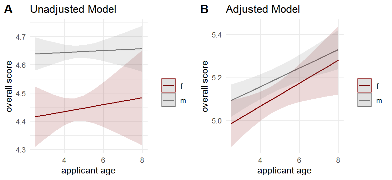
Figure 13: Interaction plot between gender and age of the applicant.

Gender of the reviewer

Table 10: Summary of a model with interaction between the applicants gender and reviewers gender, compared to the one with only main effects.

	with interaction			without interaction
(Intercept)	4.407	[4.347; 4.466]	<0.0001	4.358	[4.312; 4.405]	< 0.0001
reviewer_genderm	0.048	[-0.012; 0.109]	0.1188	0.115	[0.082; 0.148]	< 0.0001
applicant_genderm	0.128	[0.06; 0.196]	0.0002	0.195	[0.151; 0.239]	< 0.0001
reviewer_genderm:applicant_genderm	0.089	[0.021; 0.158]	0.0108	NA	NA	NA

Table 11: Summary of the model with interaction between the applicants gender and reviewers gender,

	Full model with interaction
(Intercept)	4.928	[4.812; 5.045]	<0.0001
applicant_genderm	0.033	[-0.031; 0.096]	0.3166
reviewer_genderm	0.028	[-0.03; 0.086]	0.3474
applicant_age	0.045	[0.025; 0.065]	<0.0001
applicant_affiliationETH Domain	0.112	[0.066; 0.157]	<0.0001
applicant_affiliationOther	-0.194	[-0.249; -0.139]	<0.0001
applicant_nationalityint	-0.025	[-0.059; 0.009]	0.1471
nomination_sourceother	-0.485	[-0.513; -0.458]	<0.0001
review_originnational	-0.469	[-0.503; -0.436]	<0.0001
research_topicArchitecture	0.146	[0.046; 0.246]	0.0041
research_topicBiology	0.27	[0.212; 0.329]	<0.0001
research_topicChemistry	0.24	[0.17; 0.309]	<0.0001
research_topicEconomics	-0.013	[-0.089; 0.062]	0.7304
research_topicEngineering	0.067	[0; 0.133]	0.0484
research_topicGeology	0.247	[0.144; 0.35]	<0.0001
research_topicHistory	0.322	[0.24; 0.404]	<0.0001
research_topicLinguistics	0.261	[0.183; 0.34]	<0.0001
research_topicMath./Physics	0.451	[0.385; 0.518]	<0.0001
research_topicPsychology	-0.078	[-0.152; -0.004]	0.0398
research_topicSociology	0.004	[-0.066; 0.075]	0.9041
call_cutnewer	-0.433	[-0.462; -0.404]	<0.0001
applicant_genderm:reviewer_genderm	0.07	[0.004; 0.136]	0.0374

Table 12: Analysis of Variance Table of type III of the model with gender interaction

	Chisq	Df	Pr(>Chisq)
(Intercept)	21169.302801	1	<0.001
reviewer_gender	2.433479	1	0.1188
applicant_gender	13.602843	1	<0.001
reviewer_gender:applicant_gender	6.494317	1	0.0108

Table 13: Analysis of Variance Table of type III of the model with gender interaction.

	Chisq	Df	Pr(>Chisq)
(Intercept)	6828.9826635	1	<0.001
applicant_gender	1.0029741	1	0.3166
reviewer_gender	0.8828328	1	0.3474
applicant_age	19.1894872	1	<0.001
applicant_affiliation	87.6878664	2	<0.001
applicant_nationality	2.1023656	1	0.1471
nomination_source	1191.7712630	1	<0.001
review_origin	762.7565780	1	<0.001
research_topic	352.5022649	11	<0.001
call_cut	874.2945707	1	<0.001
applicant_gender:reviewer_gender	4.3340194	1	0.0374

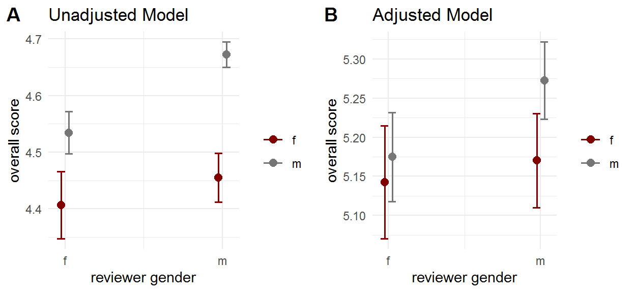
Figure 14: Interaction plot between the genders of the applicant and the reviewer.

Affilitation of the applicant

Table 14: Summary of a models with and without interaction between the applicants affilition and the applicants gender.

	with interaction			without interaction
(Intercept)	4.479	[4.431; 4.526]	<0.0001	4.434	[4.393; 4.475]	< 0.0001
applicant_affiliationETH Domain	0.198	[0.094; 0.302]	0.0002	0.284	[0.242; 0.327]	< 0.0001
applicant_affiliationOther	-0.465	[-0.57; -0.36]	<0.0001	-0.278	[-0.335; -0.221]	< 0.0001
applicant_genderm	0.105	[0.052; 0.158]	0.0001	0.163	[0.12; 0.207]	< 0.0001
applicant_affiliationETH Domain:applicant_genderm	0.107	[-0.007; 0.22]	0.0648	NA	NA	NA
applicant_affiliationOther:applicant_genderm	0.261	[0.137; 0.385]	<0.0001	NA	NA	NA

Table 15: Summary of the model with interaction between the applicants affiliation and applicants gender,

	Full model with interaction
(Intercept)	4.918	[4.805; 5.032]	<0.0001
applicant_genderm	0.046	[-0.002; 0.095]	0.0620
applicant_affiliationETH Domain	0.068	[-0.029; 0.165]	0.1718
applicant_affiliationOther	-0.334	[-0.432; -0.237]	<0.0001
reviewer_genderm	0.08	[0.048; 0.111]	<0.0001
applicant_age	0.045	[0.025; 0.066]	<0.0001
applicant_nationalityint	-0.026	[-0.06; 0.008]	0.1291
nomination_sourceother	-0.486	[-0.513; -0.458]	<0.0001
review_originnational	-0.469	[-0.503; -0.436]	<0.0001
research_topicArchitecture	0.144	[0.045; 0.244]	0.0046
research_topicBiology	0.271	[0.212; 0.329]	<0.0001
research_topicChemistry	0.24	[0.171; 0.31]	<0.0001
research_topicEconomics	-0.011	[-0.087; 0.064]	0.7680
research_topicEngineering	0.065	[-0.001; 0.131]	0.0541
research_topicGeology	0.248	[0.146; 0.351]	<0.0001
research_topicHistory	0.321	[0.238; 0.403]	<0.0001
research_topicLinguistics	0.259	[0.181; 0.338]	<0.0001
research_topicMath./Physics	0.452	[0.386; 0.519]	<0.0001
research_topicPsychology	-0.073	[-0.147; 0.001]	0.0534
research_topicSociology	0.013	[-0.058; 0.083]	0.7262
call_cutnewer	-0.432	[-0.46; -0.403]	<0.0001
applicant_genderm:applicant_affiliationETH Domain	0.056	[-0.046; 0.159]	0.2826
applicant_genderm:applicant_affiliationOther	0.196	[0.083; 0.309]	0.0007

Table 16: Analysis of Variance Table of type III of the model with affiliation interaction

	Chisq	Df	Pr(>Chisq)
(Intercept)	34615.18569	1	< 0.001
applicant_affiliation	105.53969	2	< 0.001
applicant_gender	15.08441	1	< 0.001
applicant_affiliation:applicant_gender	18.13420	2	< 0.001

Table 17: Analysis of Variance Table of type III of the model with affiliation interaction.

	Chisq	Df	Pr(>Chisq)
(Intercept)	7226.295673	1	<0.001
applicant_gender	3.482912	1	0.0620
applicant_affiliation	51.771537	2	<0.001
reviewer_gender	24.298277	1	<0.001
applicant_age	19.460799	1	<0.001
applicant_nationality	2.302993	1	0.1291
nomination_source	1194.924498	1	<0.001
review_origin	763.378115	1	<0.001
research_topic	349.924991	11	<0.001
call_cut	869.793404	1	<0.001
applicant_gender:applicant_affiliation	11.689856	2	0.0029

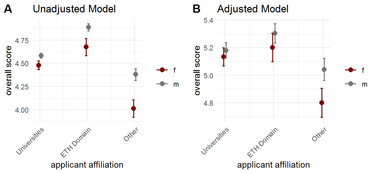
Figure 15: Interaction plot between the affiliation and the gender of the applicant.

Nationality of the applicant

Table 18: Summary of a model with interaction between the applicants nationality and the applicants gender.

	with interaction			without interaction
(Intercept)	4.427	[4.374; 4.48]	<0.0001	4.437	[4.394; 4.481]	<0.0001
applicant_nationalityint	0.033	[-0.046; 0.113]	0.4155	0.009	[-0.028; 0.046]	0.6288
applicant_genderm	0.219	[0.159; 0.278]	<0.0001	0.205	[0.161; 0.25]	<0.0001
applicant_nationalityint:applicant_genderm	-0.031	[-0.12; 0.059]	0.5058	NA	NA	NA

Table 19: Summary of the model with interaction between the applicants nationality and applicants gender,

	Full model with interaction
(Intercept)	4.888	[4.774; 5.003]	<0.0001
applicant_genderm	0.087	[0.033; 0.14]	0.0014
applicant_nationalityint	-0.022	[-0.093; 0.049]	0.5389
applicant_affiliationETH Domain	0.112	[0.066; 0.157]	<0.0001
applicant_affiliationOther	-0.194	[-0.248; -0.139]	<0.0001
reviewer_genderm	0.08	[0.048; 0.111]	<0.0001
applicant_age	0.045	[0.025; 0.065]	<0.0001
nomination_sourceother	-0.485	[-0.513; -0.458]	<0.0001
review_originnational	-0.469	[-0.503; -0.436]	<0.0001
research_topicArchitecture	0.146	[0.046; 0.246]	0.0041
research_topicBiology	0.27	[0.212; 0.329]	<0.0001
research_topicChemistry	0.241	[0.171; 0.31]	<0.0001
research_topicEconomics	-0.013	[-0.088; 0.063]	0.7445
research_topicEngineering	0.068	[0.001; 0.134]	0.0451
research_topicGeology	0.248	[0.145; 0.35]	<0.0001
research_topicHistory	0.322	[0.24; 0.404]	<0.0001
research_topicLinguistics	0.261	[0.183; 0.34]	<0.0001
research_topicMath./Physics	0.452	[0.386; 0.519]	<0.0001
research_topicPsychology	-0.076	[-0.15; -0.002]	0.0447
research_topicSociology	0.006	[-0.065; 0.076]	0.8711
call_cutnewer	-0.433	[-0.461; -0.404]	<0.0001
applicant_genderm:applicant_nationalityint	-0.004	[-0.083; 0.075]	0.9188

Table 20: Analysis of Variance Table of type III of the model with nationality interaction

	Chisq	Df	Pr(>Chisq)
(Intercept)	2.667980e+04	1	<0.001
applicant_nationality	6.629304e-01	1	0.4155
applicant_gender	5.226714e+01	1	<0.001
applicant_nationality:applicant_gender	4.427434e-01	1	0.5058

Table 21: Analysis of Variance Table of type III of the model with nationality interaction.

	Chisq	Df	Pr(>Chisq)
(Intercept)	6998.5150002	1	<0.001
applicant_gender	10.1634129	1	0.0014
applicant_nationality	0.3775390	1	0.5389
applicant_affiliation	87.2760152	2	<0.001
reviewer_gender	24.4237262	1	<0.001
applicant_age	19.3222435	1	<0.001
nomination_source	1193.5763875	1	<0.001
review_origin	763.4536462	1	<0.001
research_topic	352.2110736	11	<0.001
call_cut	873.8825783	1	<0.001
applicant_gender:applicant_nationality	0.0103907	1	0.9188

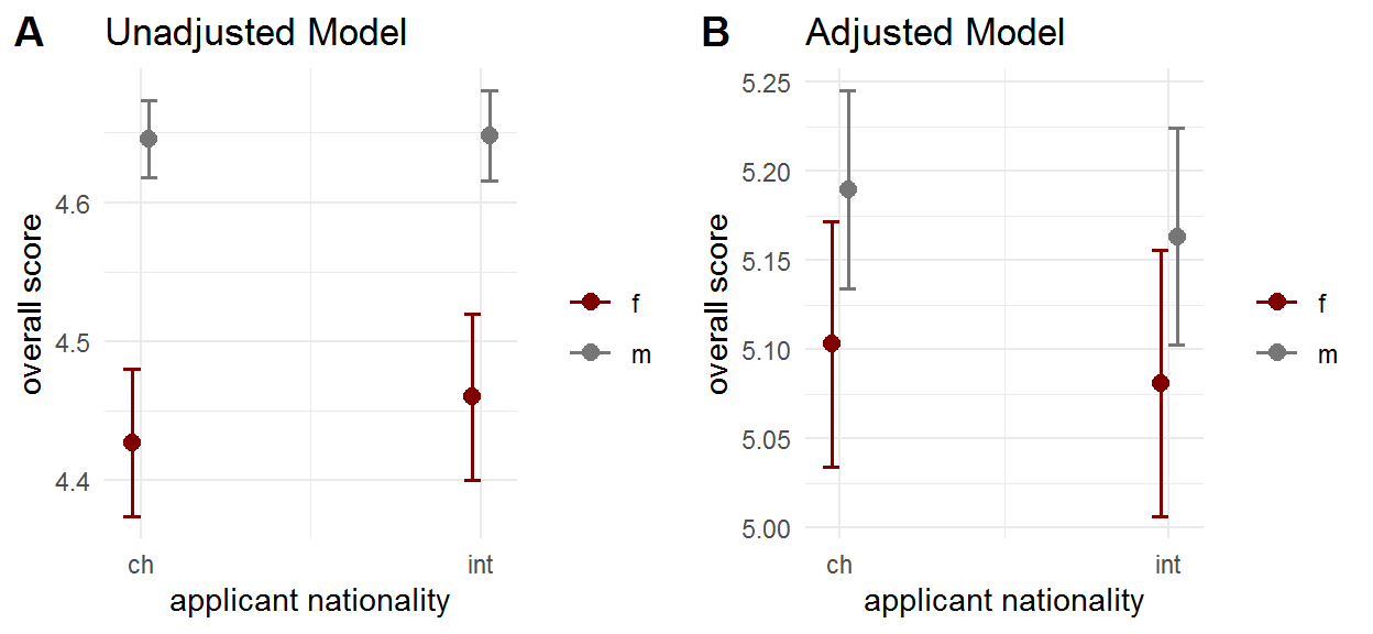
Figure 16: Interaction plot between the nationality and the gender of the applicant.

Source of nomination of the reviewer

Table 22: Summary of the models with and without interaction between the reviewer nomination source of the reviewer and the applicant`s gender.

	with interaction			without interaction
(Intercept)	4.882	[4.819; 4.946]	<0.0001	4.873	[4.829; 4.918]	< 0.0001
nomination_sourceother	-0.557	[-0.62; -0.494]	<0.0001	-0.546	[-0.574; -0.518]	< 0.0001
applicant_genderm	0.181	[0.111; 0.252]	<0.0001	0.192	[0.149; 0.235]	< 0.0001
nomination_sourceother:applicant_genderm	0.013	[-0.057; 0.083]	0.7115	NA	NA	NA

Table 23: Summary of the model with interaction between the reviewer nomination source and the applicant`s gender,

	Full model with interaction
(Intercept)	4.921	[4.801; 5.041]	<0.0001
applicant_genderm	0.047	[-0.021; 0.115]	0.1768
nomination_sourceother	-0.524	[-0.586; -0.462]	<0.0001
applicant_nationalityint	-0.025	[-0.059; 0.009]	0.1430
applicant_affiliationETH Domain	0.112	[0.066; 0.157]	<0.0001
applicant_affiliationOther	-0.194	[-0.248; -0.139]	<0.0001
reviewer_genderm	0.08	[0.048; 0.112]	<0.0001
applicant_age	0.045	[0.025; 0.065]	<0.0001
review_originnational	-0.47	[-0.503; -0.436]	<0.0001
research_topicArchitecture	0.146	[0.046; 0.246]	0.0041
research_topicBiology	0.27	[0.211; 0.329]	<0.0001
research_topicChemistry	0.241	[0.171; 0.31]	<0.0001
research_topicEconomics	-0.013	[-0.089; 0.063]	0.7364
research_topicEngineering	0.068	[0.002; 0.134]	0.0437
research_topicGeology	0.248	[0.145; 0.35]	<0.0001
research_topicHistory	0.322	[0.24; 0.404]	<0.0001
research_topicLinguistics	0.261	[0.183; 0.34]	<0.0001
research_topicMath./Physics	0.453	[0.386; 0.519]	<0.0001
research_topicPsychology	-0.076	[-0.15; -0.002]	0.0439
research_topicSociology	0.006	[-0.065; 0.076]	0.8786
call_cutnewer	-0.433	[-0.462; -0.405]	<0.0001
applicant_genderm:nomination_sourceother	0.047	[-0.021; 0.116]	0.1737

Table 24: Analysis of Variance Table of type III of the model with nomination interaction

	Chisq	Df	Pr(>Chisq)
(Intercept)	2.270657e+04	1	<0.001
nomination_source	2.994471e+02	1	<0.001
applicant_gender	2.539184e+01	1	<0.001
nomination_source:applicant_gender	1.368323e-01	1	0.7115

Table 25: Analysis of Variance Table of type III of the model with nomination interaction.

	Chisq	Df	Pr(>Chisq)
(Intercept)	6468.018730	1	<0.001
applicant_gender	1.824332	1	0.1768
nomination_source	276.061424	1	<0.001
applicant_nationality	2.145643	1	0.1430
applicant_affiliation	87.339040	2	<0.001
reviewer_gender	24.558383	1	<0.001
applicant_age	19.276241	1	<0.001
review_origin	763.951948	1	<0.001
research_topic	352.509965	11	<0.001
call_cut	875.323734	1	<0.001
applicant_gender:nomination_source	1.850528	1	0.1737

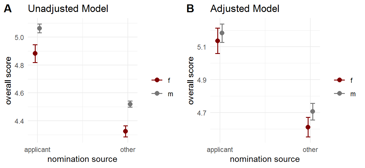
Figure 17: Interaction plot between the nomination source of the reviewer and the gender of the applicant.

Origin of the reviewer

Table 26: Summary of the models with and without interaction between the origin of the reviewer and the applicant`s gender.

	with interaction			without interaction
(Intercept)	4.542	[4.499; 4.584]	<0.0001	4.537	[4.498; 4.577]	< 0.0001
review_originnational	-0.506	[-0.57; -0.442]	<0.0001	-0.491	[-0.525; -0.456]	< 0.0001
applicant_genderm	0.192	[0.145; 0.239]	<0.0001	0.197	[0.153; 0.241]	< 0.0001
review_originnational:applicant_genderm	0.02	[-0.049; 0.088]	0.5738	NA	NA	NA

Table 27: Summary of the model with interaction between the reviewers origin source and the applicants gender,

	Full model with interaction
(Intercept)	4.897	[4.785; 5.009]	<0.0001
applicant_genderm	0.075	[0.031; 0.119]	0.0008
review_originnational	-0.499	[-0.56; -0.437]	<0.0001
nomination_sourceother	-0.486	[-0.513; -0.458]	<0.0001
applicant_nationalityint	-0.026	[-0.06; 0.008]	0.1409
applicant_affiliationETH Domain	0.112	[0.066; 0.157]	<0.0001
applicant_affiliationOther	-0.194	[-0.248; -0.139]	<0.0001
reviewer_genderm	0.08	[0.048; 0.112]	<0.0001
applicant_age	0.045	[0.025; 0.066]	<0.0001
research_topicArchitecture	0.146	[0.046; 0.246]	0.0041
research_topicBiology	0.27	[0.212; 0.329]	<0.0001
research_topicChemistry	0.241	[0.171; 0.31]	<0.0001
research_topicEconomics	-0.012	[-0.088; 0.063]	0.7500
research_topicEngineering	0.068	[0.002; 0.134]	0.0432
research_topicGeology	0.248	[0.145; 0.351]	<0.0001
research_topicHistory	0.322	[0.24; 0.404]	<0.0001
research_topicLinguistics	0.261	[0.183; 0.339]	<0.0001
research_topicMath./Physics	0.453	[0.387; 0.52]	<0.0001
research_topicPsychology	-0.076	[-0.151; -0.002]	0.0438
research_topicSociology	0.006	[-0.065; 0.077]	0.8674
call_cutnewer	-0.433	[-0.461; -0.404]	<0.0001
applicant_genderm:review_originnational	0.037	[-0.029; 0.103]	0.2669

(#tab:tab:aovORIGIN)Analysis of Variance Table of type III of the model with origin interaction

	Chisq	Df	Pr(>Chisq)
(Intercept)	4.445430e+04	1	<0.001
review_origin	2.420407e+02	1	<0.001
applicant_gender	6.339857e+01	1	<0.001
review_origin:applicant_gender	3.163514e-01	1	0.5738

Table 28: Analysis of Variance Table of type III of the model with origin interaction.

	Chisq	Df	Pr(>Chisq)
(Intercept)	7364.808805	1	<0.001
applicant_gender	11.156170	1	<0.001
review_origin	251.912641	1	<0.001
nomination_source	1194.062676	1	<0.001
applicant_nationality	2.167812	1	0.1409
applicant_affiliation	87.365257	2	<0.001
reviewer_gender	24.595771	1	<0.001
applicant_age	19.389239	1	<0.001
research_topic	352.543890	11	<0.001
call_cut	873.368021	1	<0.001
applicant_gender:review_origin	1.232856	1	0.2669

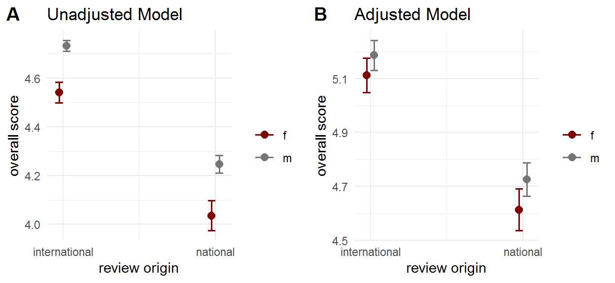
Figure 18: Interaction plot between the origin of the reviewer and the gender of the applicant.

Research topic

Table 29: Summary of models with and without interaction between the research topic and the applicant`s gender.

	with interaction			without interaction
(Intercept)	4.324	[4.247; 4.4]	<0.0001	4.316	[4.265; 4.366]	<0.0001
research_topicArchitecture	0.112	[-0.084; 0.308]	0.2624	0.068	[-0.034; 0.17]	0.1911
research_topicBiology	0.235	[0.101; 0.368]	0.0006	0.286	[0.224; 0.348]	<0.0001
research_topicChemistry	0.439	[0.272; 0.607]	<0.0001	0.447	[0.377; 0.518]	<0.0001
research_topicEconomics	-0.183	[-0.347; -0.018]	0.0294	-0.15	[-0.23; -0.069]	0.0003
research_topicEngineering	0.282	[0.119; 0.444]	0.0007	0.29	[0.227; 0.353]	<0.0001
research_topicGeology	0.573	[0.295; 0.851]	<0.0001	0.46	[0.353; 0.568]	<0.0001
research_topicHistory	0.418	[0.245; 0.591]	<0.0001	0.336	[0.249; 0.423]	<0.0001
research_topicLinguistics	0.294	[0.144; 0.444]	0.0001	0.291	[0.208; 0.375]	<0.0001
research_topicMath./Physics	0.541	[0.358; 0.724]	<0.0001	0.649	[0.582; 0.716]	<0.0001
research_topicPsychology	-0.096	[-0.227; 0.035]	0.1519	-0.155	[-0.233; -0.076]	0.0001
research_topicSociology	-0.173	[-0.302; -0.043]	0.0090	-0.081	[-0.155; -0.006]	0.0331
applicant_genderm	0.107	[0.021; 0.193]	0.0143	0.118	[0.075; 0.161]	<0.0001
research_topicArchitecture:applicant_genderm	-0.059	[-0.283; 0.165]	0.6081	NA	NA	NA
research_topicBiology:applicant_genderm	0.063	[-0.085; 0.212]	0.4017	NA	NA	NA
research_topicChemistry:applicant_genderm	0.011	[-0.172; 0.193]	0.9097	NA	NA	NA
research_topicEconomics:applicant_genderm	0.042	[-0.143; 0.228]	0.6545	NA	NA	NA
research_topicEngineering:applicant_genderm	0.011	[-0.164; 0.186]	0.9006	NA	NA	NA
research_topicGeology:applicant_genderm	-0.129	[-0.428; 0.17]	0.3967	NA	NA	NA
research_topicHistory:applicant_genderm	-0.107	[-0.301; 0.088]	0.2839	NA	NA	NA
research_topicLinguistics:applicant_genderm	-0.006	[-0.183; 0.171]	0.9510	NA	NA	NA
research_topicMath./Physics:applicant_genderm	0.122	[-0.073; 0.317]	0.2189	NA	NA	NA
research_topicPsychology:applicant_genderm	-0.098	[-0.257; 0.06]	0.2242	NA	NA	NA
research_topicSociology:applicant_genderm	0.139	[-0.015; 0.293]	0.0769	NA	NA	NA

Table 30: Summary of the model with interaction between the research topic and the applicant`s gender,

	Full model with interaction
(Intercept)	4.883	[4.759; 5.007]	<0.0001
applicant_genderm	0.094	[0.013; 0.175]	0.0223
research_topicArchitecture	0.236	[0.05; 0.422]	0.0131
research_topicBiology	0.19	[0.064; 0.316]	0.0031
research_topicChemistry	0.226	[0.068; 0.385]	0.0052
research_topicEconomics	-0.008	[-0.163; 0.146]	0.9158
research_topicEngineering	0.108	[-0.048; 0.263]	0.1745
research_topicGeology	0.359	[0.097; 0.62]	0.0071
research_topicHistory	0.427	[0.265; 0.59]	<0.0001
research_topicLinguistics	0.289	[0.148; 0.43]	<0.0001
research_topicMath./Physics	0.377	[0.205; 0.549]	<0.0001
research_topicPsychology	-0.013	[-0.137; 0.11]	0.8310
research_topicSociology	-0.034	[-0.157; 0.088]	0.5832
review_originnational	-0.47	[-0.503; -0.436]	<0.0001
nomination_sourceother	-0.485	[-0.513; -0.458]	<0.0001
applicant_nationalityint	-0.025	[-0.059; 0.009]	0.1511
applicant_affiliationETH Domain	0.112	[0.066; 0.157]	<0.0001
applicant_affiliationOther	-0.192	[-0.247; -0.138]	<0.0001
reviewer_genderm	0.08	[0.048; 0.112]	<0.0001
applicant_age	0.045	[0.025; 0.065]	<0.0001
call_cutnewer	-0.434	[-0.462; -0.405]	<0.0001
applicant_genderm:research_topicArchitecture	-0.12	[-0.33; 0.09]	0.2638
applicant_genderm:research_topicBiology	0.098	[-0.041; 0.238]	0.1663
applicant_genderm:research_topicChemistry	0.016	[-0.155; 0.187]	0.8520
applicant_genderm:research_topicEconomics	-0.006	[-0.18; 0.168]	0.9478
applicant_genderm:research_topicEngineering	-0.047	[-0.211; 0.117]	0.5764
applicant_genderm:research_topicGeology	-0.129	[-0.409; 0.151]	0.3674
applicant_genderm:research_topicHistory	-0.137	[-0.32; 0.046]	0.1414
applicant_genderm:research_topicLinguistics	-0.039	[-0.205; 0.126]	0.6407
applicant_genderm:research_topicMath./Physics	0.083	[-0.099; 0.265]	0.3708
applicant_genderm:research_topicPsychology	-0.099	[-0.248; 0.049]	0.1908
applicant_genderm:research_topicSociology	0.063	[-0.082; 0.208]	0.3931

Table 31: Analysis of Variance Table of type III of the model with research topic interaction

	Chisq	Df	Pr(>Chisq)
(Intercept)	12239.125433	1	<0.001
research_topic	153.509057	11	<0.001
applicant_gender	5.994573	1	0.0143
research_topic:applicant_gender	12.002317	11	0.3635

Table 32: Analysis of Variance Table of type III of the model with topic interaction.

	Chisq	Df	Pr(>Chisq)
(Intercept)	5965.815269	1	<0.001
applicant_gender	5.221376	1	0.0223
research_topic	74.130234	11	<0.001
review_origin	763.541634	1	<0.001
nomination_source	1192.902703	1	<0.001
applicant_nationality	2.061255	1	0.1511
applicant_affiliation	86.399003	2	<0.001
reviewer_gender	24.545070	1	<0.001
applicant_age	19.143441	1	<0.001
call_cut	875.275071	1	<0.001
applicant_gender:research_topic	12.796594	11	0.3068

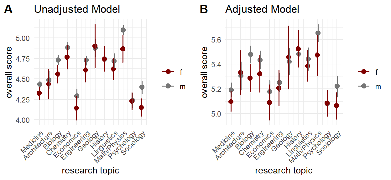
Figure 19: Interaction plot between the research topic and the gender of the applicant.

Guidelines

Table 33: Summary of models with and without an interaction between the guidelines and the applicant`s gender.

	with interaction			without interaction
(Intercept)	4.809	[4.745; 4.873]	<0.0001	4.766	[4.722; 4.811]	< 0.0001
call_cutnewer	-0.49	[-0.558; -0.423]	<0.0001	-0.433	[-0.462; -0.404]	< 0.0001
applicant_genderm	0.133	[0.063; 0.203]	0.0002	0.185	[0.141; 0.229]	< 0.0001
call_cutnewer:applicant_genderm	0.071	[-0.004; 0.146]	0.0653	NA	NA	NA

Table 34: Summary of the model with interaction between the guidelines and the applicant`s gender.

	Full model with interaction
(Intercept)	4.937	[4.818; 5.056]	<0.0001
call_cutnewer	-0.497	[-0.562; -0.431]	<0.0001
applicant_genderm	0.028	[-0.039; 0.094]	0.4157
research_topicArchitecture	0.148	[0.048; 0.247]	0.0037
research_topicBiology	0.27	[0.211; 0.328]	<0.0001
research_topicChemistry	0.24	[0.171; 0.31]	<0.0001
research_topicEconomics	-0.012	[-0.087; 0.064]	0.7654
research_topicEngineering	0.068	[0.002; 0.134]	0.0427
research_topicGeology	0.248	[0.146; 0.351]	<0.0001
research_topicHistory	0.323	[0.241; 0.405]	<0.0001
research_topicLinguistics	0.263	[0.184; 0.341]	<0.0001
research_topicMath./Physics	0.453	[0.386; 0.519]	<0.0001
research_topicPsychology	-0.075	[-0.149; -0.001]	0.0479
research_topicSociology	0.008	[-0.062; 0.079]	0.8180
review_originnational	-0.469	[-0.503; -0.436]	<0.0001
nomination_sourceother	-0.486	[-0.513; -0.458]	<0.0001
applicant_nationalityint	-0.025	[-0.059; 0.009]	0.1426
applicant_affiliationETH Domain	0.112	[0.067; 0.158]	<0.0001
applicant_affiliationOther	-0.192	[-0.247; -0.137]	<0.0001
reviewer_genderm	0.08	[0.048; 0.111]	<0.0001
applicant_age	0.045	[0.025; 0.065]	<0.0001
call_cutnewer:applicant_genderm	0.079	[0.006; 0.151]	0.0327

Table 35: Analysis of Variance Table of type III of the model with guideline interaction

	Chisq	Df	Pr(>Chisq)
(Intercept)	21855.555518	1	<0.001
call_cut	200.936308	1	<0.001
applicant_gender	13.906608	1	<0.001
call_cut:applicant_gender	3.396798	1	0.0653

Table 36: Analysis of Variance Table of type III of the model with guideline interaction.

	Chisq	Df	Pr(>Chisq)
(Intercept)	6586.4669816	1	<0.001
call_cut	221.8009368	1	<0.001
applicant_gender	0.6625622	1	0.4157
research_topic	351.4740681	11	<0.001
review_origin	763.3967105	1	<0.001
nomination_source	1195.8883272	1	<0.001
applicant_nationality	2.1499120	1	0.1426
applicant_affiliation	86.8462527	2	<0.001
reviewer_gender	24.3404171	1	<0.001
applicant_age	19.2801041	1	<0.001
call_cut:applicant_gender	4.5596998	1	0.0327

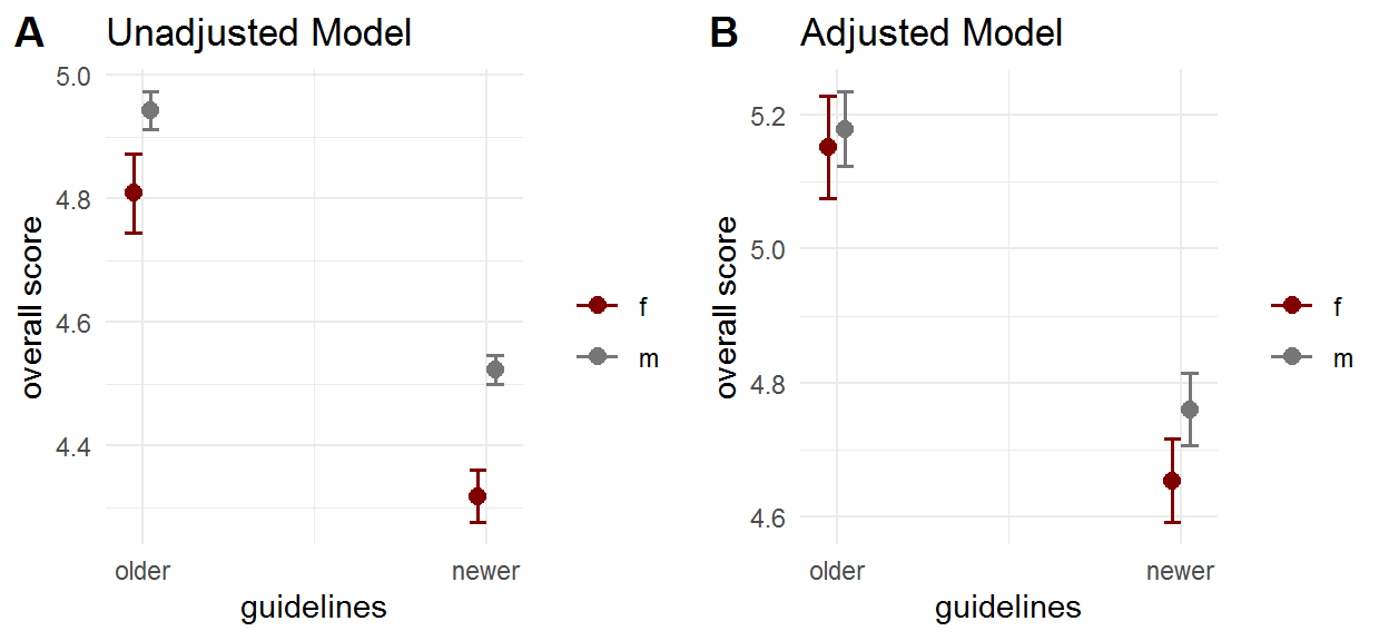
Figure 20: Interaction plot between the guidelines and the gender of the applicant.

Acknowledgments

We are grateful to Andreas Limacher (Clinical Trials Unit of the Faculty of Medicine of the University of Bern) for guiding us with the methodology.

Statistics by Research Topic

Given the differences between average scores per research topic, we examine how these differences unfold according to other variables. Figure 21 highlights the importance of looking at the effect of one variable in the context of other variables. In this case, it highlights the importance of adjusting for the topic of research when looking at gender effects. On the left panel, we see that how the average scores correlates with the percentage of female applicants for each topic. Female applicants are minority in every topic. Disciplines such as Mathematics and Physics count with as little as 10% female applicants whereas Psychology counts with up to about 40% female applicants. As expected, topics with higher shares of female applicants tend to have lower average scores. On the right panel, we try to locate unusual interactions between the gender of applicants and of reviewers in terms of average scores per topic. In psychology, for instance, male reviewers attributed significantly lower scores to female applicants, whereas in sociology female applicants were penalized by female reviewers. Most differences were nevertheless not significant.

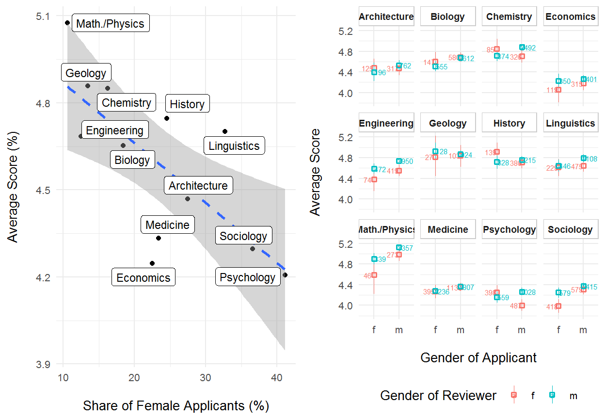
Figure 21: Left panel: scatter plot showing the average review scores versus the percentage of female applicants for each research topic. Blue dotted line and the shaded area show the slope and 95% confidence interval of a linear model on the scatter points. Right panel: mean review scores per research topic, per gender of the applicant (f: female applicant, m: male applicant), and per gender of the reviewer (f: female reviewers in red, m: male reviewers in blue). Text annotations show the number of observations and bars show the 95% confidence intervals of the mean.

In Figure 22, we check whether the percentage of female reviewers correlates that of female applicants, and whether the percentage Swiss-based reviews correlates with that of Swiss applicants. As we can see on the left panel, female applicants tend to be slightly underrepresented in terms of female reviewers: though differences are small, 9 over 12 research topics have somewhat smaller percentages of female reviewers than of female applicants. Then, on the right panel, we can see that, with the exception of Economics and Linguistics, topics with higher percentages of Swiss applicants also tend to receive higher percentages of reviews from within Switzerland.

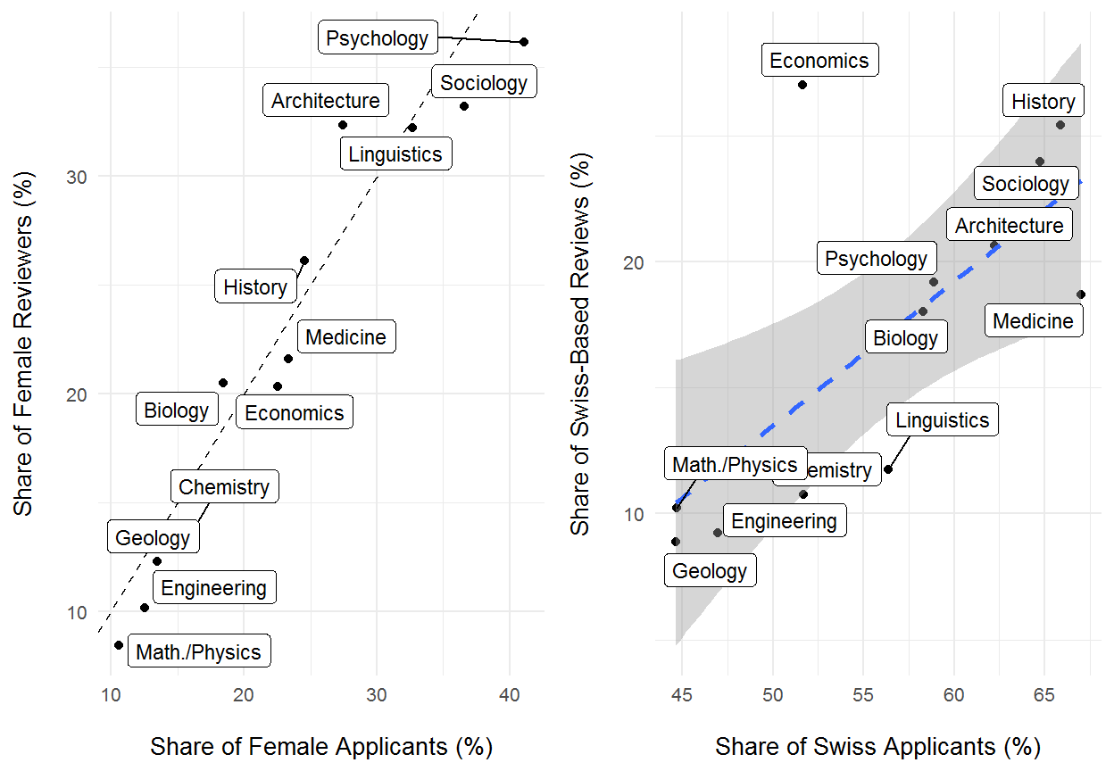
Figure 22: Left panel: scatter plot showing the share of male reviewers versus the share of female applicants for each research topic. The dotted line shows the identity line. Right panel : scatter plot showing the percentage of Swiss-based reviews versus the percentage of Swiss applicants for each research topic. The blue dotted line and the shaded areas show the slope and 95% confidence interval of a linear model of the points.

Final Remarks

For the regression models, we choose to show the age of the applicants (applicant_age) in decades to improve the magnitude and the ease of interpretation of age effects in the regression models. We introduce a dummy variable (call_cut) to capture the introduction of new, stricter, SNSF guidelines for reviewers in the call of October 2011. Due to stricter reviewing guidelines, grant applications submitted after the call of April 2011 receive significantly lower scores than earlier grant applications (see Figure 12).

Bates, Douglas, Martin Mächler, Ben Bolker, and Steve Walker. 2015. “Fitting Linear Mixed-Effects Models Using lme4.” Journal of Statistical Software 67 (1): 1–48. https://doi.org/10.18637/jss.v067.i01.

Christensen, R. H. B. 2018. “Ordinal—Regression Models for Ordinal Data.” http://www.cran.r-project.org/package=ordinal.

Harrison, Xavier A, Lynda Donaldson, Maria Eugenia Correa-Cano, Julian Evans, David N Fisher, Cecily Goodwin, Beth Robinson, David J Hodgson, and Richard Inger. 2018. “A Brief Introduction to Mixed Effects Modelling and Multi-Model Inference in Ecology.” PeerJ 6:E4794. https://doi.org/10.7717/peerj.4794.